YAP: Yet Another Probabilistic Neural Network

By the end of 2019, I finally managed to wrap up my third R package YAP (https://github.com/statcompute/yap) that implements the Probabilistic Neural Network (Specht, 1990) for the N-category pattern recognition with N > 2. Similar to GRNN, PNN shares same benefits of instantaneous training, simple structure, and global convergence.

Below is a demonstration showing how to use the YAP package and a comparison between the multinomial regression and the PNN. As shown below, both approaches delivered very comparable predictive performance. In this particular example, PNN even performed slightly better in terms of the cross-entropy for a separate testing dataset.

data("Heating", package = "mlogit")
Y <- Heating[, 2]
X <- scale(Heating[, 3:15])
idx <- with(set.seed(1), sample(seq(nrow(X)), nrow(X) / 2))

### FIT A MULTINOMIAL REGRESSION AS A BENCHMARK ###
m1 <- nnet::multinom(Y ~ ., data = data.frame(X, Y)[idx, ], model = TRUE)
# cross-entropy for the testing set
yap::logl(y_pred = predict(m1, newdata = X, type = "prob")[-idx, ], y_true = yap::dummies(Y)[-idx, ])
# 1.182727

### FIT A PNN ###
n1 <- yap::pnn.fit(x = X[idx, ], y = Y[idx])
parm <- yap::pnn.search_logl(n1, yap::gen_latin(1, 10, 20), nfolds = 5)
n2 <- yap::pnn.fit(X[idx, ], Y[idx], sigma = parm$best$sigma)
# cross-entropy for the testing set
yap::logl(y_pred = yap::pnn.predict(n2, X)[-idx, ], y_true = yap::dummies(Y)[-idx, ])
# 1.148456

Improve General Regression Neural Network by Monotonic Binning

A major criticism on the binning algorithm as well as on the WoE transformation is that the use of binned predictors will decrease the model predictive power due to the loss of data granularity after the WoE transformation. While talk is cheap, I would use the example below to show that using the monotonic binning algorithm to pre-process predictors in a GRNN is actually able to alleviate the over-fitting and to improve the prediction accuracy for the hold-out sample.

First of all, the whole dataset was split into half, e.g. one as the training sample and another as the hold-out sample. The smoothing parameter, e.g. sigma, was chosen through the random search and happened to be 2.198381 for both GRNNs.

1. For the first GRNN with untransformed raw predictors, the AUC for the training sample is 0.69 and the AUC for the hold-out sample is 0.66.
2. For the second GRNN with WoE-transformed predictors, the AUC for the training sample is 0.72 and the AUC for the hold-out sample is 0.69.

In this particular example, it is clearly shown that there is roughly a 4% – 5% improvement in the AUC statistic for both training and hold-out samples through the use of monotonic binning and WoE transformations.

	df1 <- read.table("credit_count.txt", header = T, sep = ",")
	df2 <- df1[which(df1$CARDHLDR == 1), ]
	Y <- df2$DEFAULT
	X <- scale(df2[, 3:ncol(df2)])
	i <- sample(seq(length(Y)), length(Y) / 2)
	# WITHOUT BINNING
	Y1 <- Y[i]
	Y2 <- Y[-i]
	X1 <- X[i, ]
	X2 <- X[-i, ]
	net11 <- grnn.fit(x = X1, y = Y1)
	test1 <- grnn.search_auc(net11, gen_latin(1, 3, 10), nfolds = 4)
	# $best
	# sigma auc
	# 2.198381 0.6297201
	net12 <- grnn.fit(x = X1, y = Y1, sigma = test1$best$sigma)
	MLmetrics::AUC(grnn.parpred(net12, X1), Y1)
	# 0.6855638
	MLmetrics::AUC(grnn.parpred(net12, X2), Y2)
	# 0.6555798
	# WITH BINNING
	df3 <- data.frame(df2[, 3:ncol(df2)], Y)
	bin_out <- batch_bin(df3, method = 3)
	df_woe <- batch_woe(df3, bin_out$BinLst)
	W <- scale(df_woe$df[, -1])
	W1 <- W[i, ]
	W2 <- W[-i, ]
	net21 <- grnn.fit(x = W1, y = Y1)
	test2 <- grnn.search_auc(net21, gen_latin(1, 3, 10), nfolds = 4)
	# $best
	# sigma auc
	# 2.198381 0.6820317
	net22 <- grnn.fit(x = W1, y = Y1, sigma = test2$best$sigma)
	MLmetrics::AUC(grnn.parpred(net22, W1), Y1)
	# 0.7150051
	MLmetrics::AUC(grnn.parpred(net22, W2), Y2)
	# 0.6884229

view raw

grnn_bin.R

hosted with ❤ by GitHub

GRNN with Small Samples

After a bank launches a new product or acquires a new portfolio, the risk modeling team would often be faced with a challenge of how to estimate the corresponding performance, e.g. risk or loss, with a limited number of data points conditional on business drivers or macro-economic indicators. For instance, it is required to project the 9-quarter loss in CCAR, regardless of the portfolio age. In such cases, the prevalent practice based upon conventional regression models might not be applicable given the requirement for a sufficient number of samples in order to draw the statistical inference. As a result, we would have to rely on the input of SME (Subject Matter Expert), to gauge the performance based on similar products and portfolios, or to fall back on simple statistical metrics such as Average or Median that can’t be intuitively related to predictors.

With the GRNN implemented in the YAGeR project (https://github.com/statcompute/yager), it is however technically feasible to project the expected performance conditional on predictors due to the fact that the projected Y_i of a future case is determined by the distance between the predictor vector X_i and each X vector in the training sample, subject to a smoothing parameter namely Sigma. While more samples in the training data are certainly helpful to estimate a generalizable model, a couple data points, e.g. even only one or two data points in the extreme case, are also conceptually sufficient to form a GRNN that is able to generate sensible projections without violating statistical assumptions.

Following are a couple practical considerations.

1. Although normalizing the input data, e.g. X matrix, in a GRNN is usually necessary for the numerical reason, the exact scaling is not required. Practically, the “rough” scaling can be employed and ranges or variances used in the normalization can be based upon the historical data of X that might not be reflected in the training data with only a small sample size.
2. With limited data points in the training data, the Sigma value can be chosen by the L-O-O (Leave-One-Out) or empirically based upon another GRNN with a similar data structure that might or might not be related to the training data. What’s more, it is easy enough to dynamically fine-tune or refresh the Sigma value with more data samples becoming available along the time.
3. While there is no requirement for the variable selection in a GRNN, the model developer does have the flexibility of judgmentally choosing predictors based upon the prior information and eliminating variables not showing correct marginal effects in PDP (https://statcompute.wordpress.com/2019/10/19/partial-dependence-plot-pdp-of-grnn).

Below is an example of using 100 data points as the training sample to predict LGD within the unity interval of 1,000 cases with both GLM and GRNN. Out of 100 trials, while the GLM only outperformed the simple average for 32 times, the GRNN was able to do better for 76 times.

	source("yager.R")
	df <- read.table("lgd", header = T)[, 1:8]
	Y <- 1 – df$rr
	X <- scale(df[, 2:8])
	pre.N <- 1000
	trn.N <- 100
	try.N <- 100
	seeds <- floor(with(set.seed(2020), runif(try.N) * 1e8))
	test_glm <- function(seed) {
	i1 <- with(set.seed(seed), sample(seq(length(Y)), pre.N))
	Y1 <- Y[i1]
	X1 <- X[i1, ]
	Y2 <- Y[-i1]
	X2 <- X[-i1, ]
	i2 <- with(set.seed(seed), sample(seq(length(Y2)), trn.N))
	gm <- glm(Y2 ~ ., data = data.frame(Y2, X2)[i2, ], family = quasibinomial)
	round(MLmetrics::R2_Score(predict(gm, newdata = data.frame(X1), type = "response"), Y1), 4)
	}
	perf.glm <- Reduce(c, lapply(seeds, test_glm))
	summary(perf.glm)
	# Min. 1st Qu. Median Mean 3rd Qu. Max.
	# -0.39300 -0.10483 -0.02280 -0.05135 0.01230 0.08920
	sum(perf.glm > 0) / length(perf.glm)
	# [1] 0.32
	test_grnn <- function(seed) {
	i1 <- with(set.seed(seed), sample(seq(length(Y)), pre.N))
	Y1 <- Y[i1]
	X1 <- X[i1, ]
	Y2 <- Y[-i1]
	X2 <- X[-i1, ]
	i2 <- with(set.seed(seed), sample(seq(length(Y2)), trn.N))
	gn <- grnn.fit(X2[i2, ], Y2[i2])
	round(MLmetrics::R2_Score(grnn.predict(gn, X1), Y1), 4)
	}
	perf.grnn <- Reduce(c, lapply(seeds, test_grnn))
	summary(perf.grnn)
	# Min. 1st Qu. Median Mean 3rd Qu. Max.
	# -0.06130 0.00075 0.03075 0.02739 0.05437 0.10000
	sum(perf.grnn > 0) / length(perf.grnn)
	# [1] 0.76

view raw

grnn_SmallSample.R

hosted with ❤ by GitHub

GRNN vs. GAM

In practice, GRNN is very similar to GAM (Generalized Additive Models) in the sense that they both shared the flexibility of approximating non-linear functions. In the example below, both GRNN and GAM were applied to the Kyphosis data that has been widely experimented in examples of GAM and revealed very similar patterns of functional relationships between model predictors and the response (red for GRNN and blue for GAM). However, while we have to determine the degree of freedom for each predictor in order to control the smoothness of a GAM model, there is only one tuning parameter governing the overall fitting of a GRNN model.

	data(kyphosis, package = "gam")
	y <- ifelse(kyphosis$Kyphosis == "present", 1, 0)
	x <- scale(kyphosis[, -1])
	### FIT A GRNN
	net1 <- grnn.fit(x = x, y = y)
	test <- grnn.search_auc(net1, sigmas = gen_sobol(min = 0.5, max = 1.5, n = 50), nfolds = 20)
	net2 <- grnn.fit(x = x, y = y, sigma = min(test$best$sigma))
	### FIT A GAM
	library(gam)
	gam1 <- gam(y~ Age + Number + Start, data = data.frame(y, x), family = binomial)
	step <- step.Gam(gam1, data = data.frame(x, y), direction = "both",
	scope = list("Age" = ~1 + Age + s(Age, 3) + s(Age, 4) + s(Age, 5),
	"Number" = ~1 + Number + s(Number, 3) + s(Number, 4) + s(Number, 5),
	"Start" = ~1 + Start + s(Start, 3)+ s(Start, 4) + s(Start, 5)))
	# Start: y ~ Age + Number + Start; AIC= 69.3799
	# Step:1 y ~ s(Age, 3) + Number + Start ; AIC= 66.1469
	# Step:2 y ~ s(Age, 3) + Number + s(Start, 3) ; AIC= 64.1875
	gam2 <- gam::gam(y ~ s(Age, 3) + Number + s(Start, 3), data = data.frame(x, y), family = binomial)
	### PLOTTING
	par(mfrow = c(2, 3))
	for (i in 1:ncol(net2$x)) grnn.margin(net2, i)
	plot(gam2, col = "blue", lwd = 5)

view raw

compare_gam.R

hosted with ❤ by GitHub

Permutation Feature Importance (PFI) of GRNN

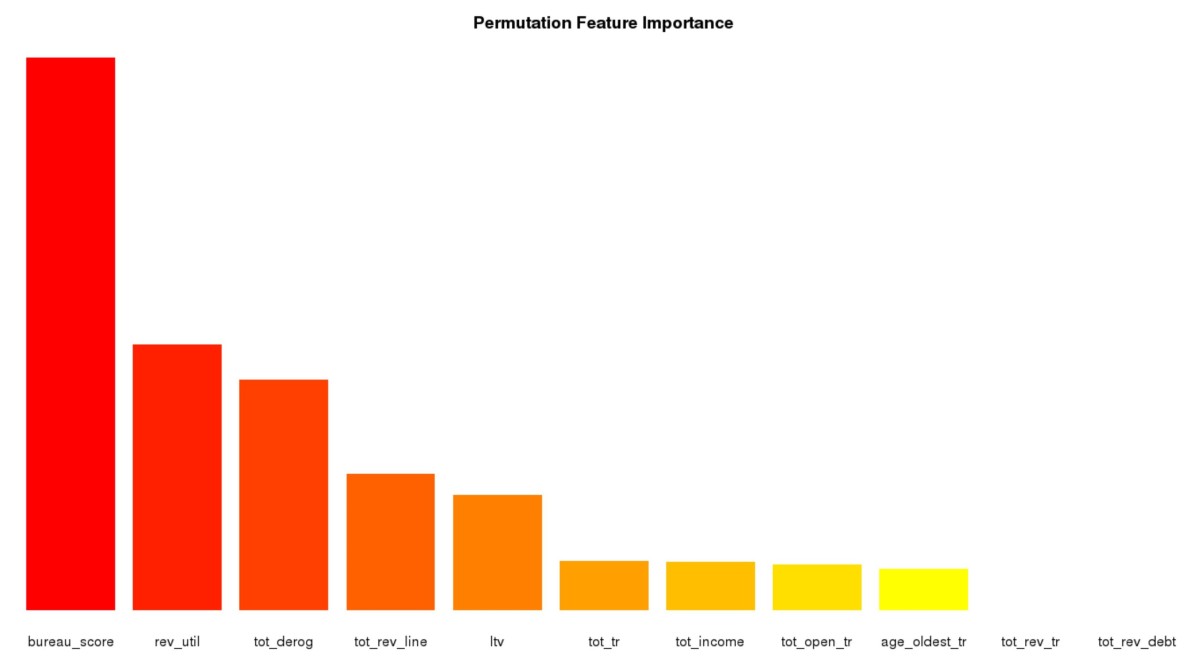
In the post https://statcompute.wordpress.com/2019/10/13/assess-variable-importance-in-grnn, it was shown how to assess the variable importance of a GRNN by the decrease in GoF statistics, e.g. AUC, after averaging or dropping the variable of interest. The permutation feature importance evaluates the variable importance in a similar manner by permuting values of the variable, which attempts to break the relationship between the predictor and the response.

Today, I added two functions to calculate PFI in the YAGeR project, e.g. the grnn.x_pfi() function (https://github.com/statcompute/yager/blob/master/code/grnn.x_pfi.R) calculating PFI of an individual variable and the grnn.pfi() function (https://github.com/statcompute/yager/blob/master/code/grnn.pfi.R) calculating PFI for all variables in the GRNN.

Below is an example showing how to use PFI to evaluate the variable importance. It turns out that the outcome looks very similar to the one created by the grnn.imp() function previously discussed.

	### INITIATE A GRNN
	net1 <- grnn.fit(x = X1, y = Y1)
	### FIND THE OPTIMIZED PARAMETER
	best <- grnn.optmiz_auc(net1, lower = 1, upper = 3)
	### FIT A GRNN WITH THE OPTIMIZED PARAMETER
	net2 <- grnn.fit(x = X1, y = Y1, sigma = best$sigma)
	### CALCULATE PFI BY TRYING 1000 RANDOM PERMUTATIONS
	pfi_rank <- grnn.pfi(net2, ntry = 1000)
	# idx var pfi
	# 9 woe.bureau_score 0.06821683
	# 8 woe.rev_util 0.03277195
	# 1 woe.tot_derog 0.02845173
	# 7 woe.tot_rev_line 0.01680968
	# 10 woe.ltv 0.01416647
	# 2 woe.tot_tr 0.00610415
	# 11 woe.tot_income 0.00595962
	# 4 woe.tot_open_tr 0.00561115
	# 3 woe.age_oldest_tr 0.00508052
	# 5 woe.tot_rev_tr 0.00000000
	# 6 woe.tot_rev_debt 0.00000000
	### PLOT PFI
	barplot(pfi_rank$pfi, beside = TRUE, col = heat.colors(nrow(pfi_rank)), border = NA, yaxt = "n",
	names.arg = substring(pfi_rank$var, 5), main = "Permutation Feature Importance")
	### EXTRACT VARIABLES WITH 0 PFI
	excol <- pfi_rank[pfi_rank$pfi == 0, ]$idx
	# 5 6
	### AUC FOR HOLD-OUT SAMPLE WITH ALL VARIABLES
	MLmetrics::AUC(y_pred = grnn.parpred(grnn.fit(x = X1, y = Y1, sigma = best$sigma), X2), y_true = Y2)
	# 0.7584476
	### AUC FOR HOLD-OUT SAMPLE WITH PFI > 0 VARIABLES
	MLmetrics::AUC(y_pred = grnn.parpred(grnn.fit(x = X1[, -excol], y = Y1, sigma = best$sigma), X2[, -excol]), y_true = Y2)
	# 0.7622679

view raw

use_pfi.R

hosted with ❤ by GitHub

Partial Dependence Plot (PDP) of GRNN

The function grnn.margin() (https://github.com/statcompute/yager/blob/master/code/grnn.margin.R) was my first attempt to explore the relationship between each predictor and the response in a General Regression Neural Network, which usually is considered the Black-Box model. The idea is described below:

1. First trained a GRNN with the original training dataset
2. Created an artificial dataset from the training data by keeping distinct values of the variable that we are interested in but replacing all values of other variables with their means. For instance, given a dataset with three variables X1, X2, and X3, if we are interested in the marginal effect of X1 with 3 distinct values, e.g. [X11 X12 X13], then the constructed dataset should look like {[X11 mean(X2) mean(X3)], [X12 mean(X2) mean(X3)], [X13 mean(X2) mean(X3)]}
3. Calculated predicted values, namely [Pred1 Pred2 Pred3], based on the constructed dataset by using the GRNN created in the first step
4. At last, the relationship between [X11 X12 X13] and [Pred1 Pred2 Pred3] is what we are looking for

The above-mentioned approach is computationally efficient but might be somewhat “brutal” in a sense that it doesn’t consider the variation in other variables.

By the end of Friday, my boss pointed me to a paper describing the partial dependence plot (Yes! In 53, we also have SVP who is technically savvy). The idea is very intriguing, albeit computationally expensive, and is delineated as below:

1. First trained a GRNN with the original training dataset
2. Based on the training dataset, get a list of distinct values from the variable of interest, e.g. [X11 X12 X13]. In this particular example, we created three separate datasets from the training data by keeping the other variables as they are but replacing all values of X1 with each of [X11 X12 X13] respectively
3. With each of three constructed datasets above, calculated predicted values and then averaged them out such that we would have an average of predicted values for each of [X11 X12 X13], namely [Pavg1 Pavg2 Pavg3]
4. The relationship between [X11 X12 X13] and [Pavg1 Pavg2 Pavg3] is the so-called Partial Dependence

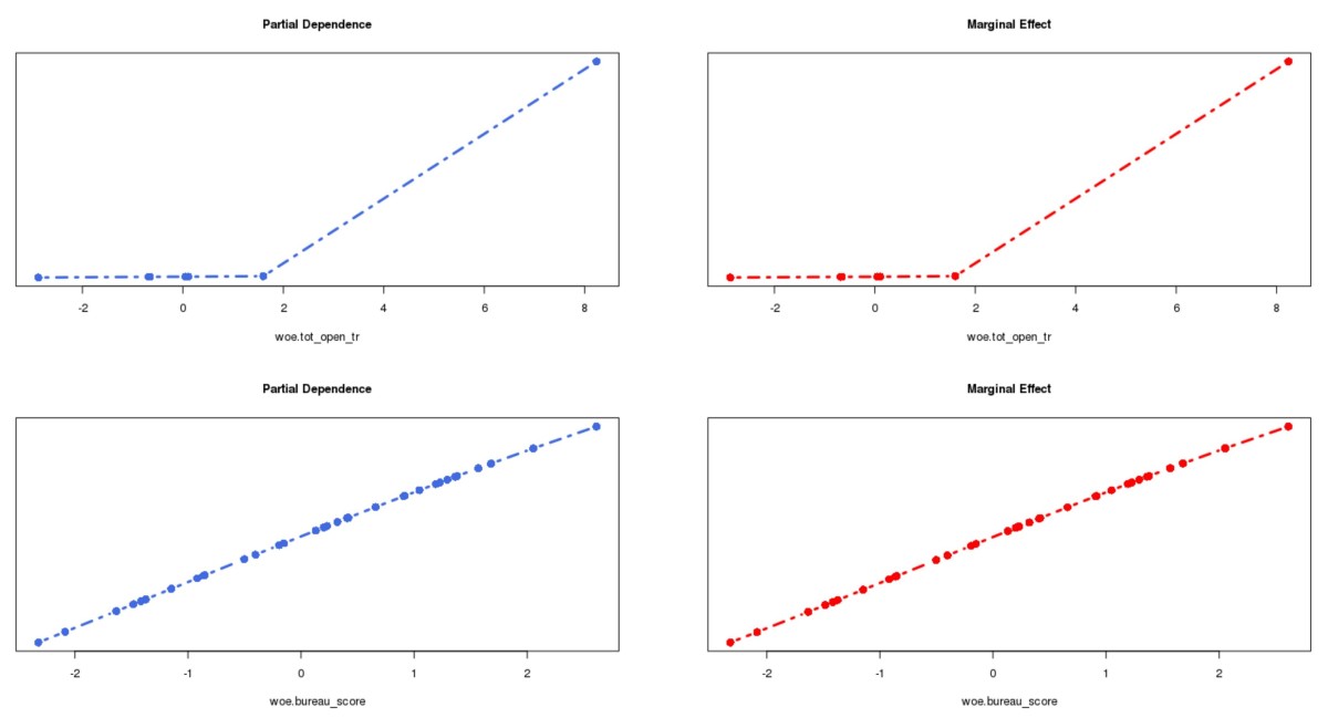
The idea of PDP has been embedded in the YAGeR project (https://github.com/statcompute/yager/blob/master/code/grnn.partial.R). In the chart below, I compared outcomes of grnn.partial() and grnn.margin() side by side for two variables, e.g. the first not so predictive and the second very predictive. In this particular comparison, both appeared almost identical.

Merge MLP And CNN in Keras

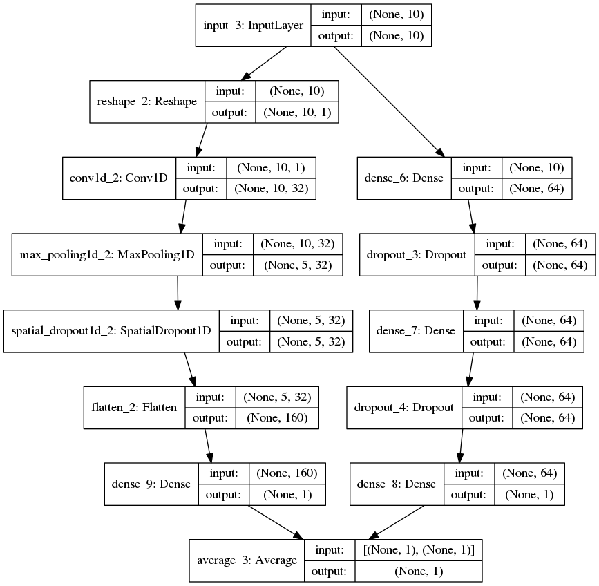
In the post (https://statcompute.wordpress.com/2017/01/08/an-example-of-merge-layer-in-keras), it was shown how to build a merge-layer DNN by using the Keras Sequential model. In the example below, I tried to scratch a merge-layer DNN with the Keras functional API in both R and Python. In particular, the merge-layer DNN is the average of a multilayer perceptron network and a 1D convolutional network, just for fun and curiosity. Since the purpose of this exercise is to explore the network structure and the use case of Keras API, I didn’t bother to mess around with parameters.

	library(keras)
	df <- read.csv("credit_count.txt")
	Y <- matrix(df[df$CARDHLDR == 1, ]$DEFAULT)
	X <- scale(df[df$CARDHLDR == 1, ][3:14])
	inputs <- layer_input(shape = c(ncol(X)))
	mlp <- inputs %>%
	layer_dense(units = 64, activation = 'relu', kernel_initializer = 'he_uniform') %>%
	layer_dropout(rate = 0.2, seed = 1) %>%
	layer_dense(units = 64, activation = 'relu', kernel_initializer = 'he_uniform') %>%
	layer_dropout(rate = 0.2, seed = 1) %>%
	layer_dense(1, activation = 'sigmoid')
	cnv <- inputs %>%
	layer_reshape(c(ncol(X), 1)) %>%
	layer_conv_1d(32, 4, activation = 'relu', padding = "same", kernel_initializer = 'he_uniform') %>%
	layer_max_pooling_1d(2) %>%
	layer_spatial_dropout_1d(0.2) %>%
	layer_flatten() %>%
	layer_dense(1, activation = 'sigmoid')
	avg <- layer_average(c(mlp, cnv))
	mdl <- keras_model(inputs = inputs, outputs = avg)
	mdl %>% compile(optimizer = optimizer_sgd(lr = 0.1, momentum = 0.9), loss = 'binary_crossentropy', metrics = c('binary_accuracy'))
	mdl %>% fit(x = X, y = Y, epochs = 50, batch_size = 1000, verbose = 0)
	mdl %>% predict(x = X)

view raw

keras_average.R

hosted with ❤ by GitHub

	from numpy.random import seed
	from pandas import read_csv, DataFrame
	from sklearn.preprocessing import scale
	from keras.layers.convolutional import Conv1D, MaxPooling1D
	from keras.layers.merge import average
	from keras.layers import Input, Dense, Flatten, Reshape, Dropout, SpatialDropout1D
	from keras.models import Model
	from keras.optimizers import SGD
	from keras.utils import plot_model
	df = read_csv("credit_count.txt")
	Y = df[df.CARDHLDR == 1].DEFAULT
	X = scale(df[df.CARDHLDR == 1].iloc[:, 2:12])
	D = 0.2
	S = 1
	seed(S)
	### INPUT DATA
	inputs = Input(shape = (X.shape[1],))
	### DEFINE A MULTILAYER PERCEPTRON NETWORK
	mlp_net = Dense(64, activation = 'relu', kernel_initializer = 'he_uniform')(inputs)
	mlp_net = Dropout(rate = D, seed = S)(mlp_net)
	mlp_net = Dense(64, activation = 'relu', kernel_initializer = 'he_uniform')(mlp_net)
	mlp_net = Dropout(rate = D, seed = S)(mlp_net)
	mlp_out = Dense(1, activation = 'sigmoid')(mlp_net)
	mlp_mdl = Model(inputs = inputs, outputs = mlp_out)
	### DEFINE A CONVOLUTIONAL NETWORK
	cnv_net = Reshape((X.shape[1], 1))(inputs)
	cnv_net = Conv1D(32, 4, activation = 'relu', padding = "same", kernel_initializer = 'he_uniform')(cnv_net)
	cnv_net = MaxPooling1D(2)(cnv_net)
	cnv_net = SpatialDropout1D(D)(cnv_net)
	cnv_net = Flatten()(cnv_net)
	cnv_out = Dense(1, activation = 'sigmoid')(cnv_net)
	cnv_mdl = Model(inputs = inputs, outputs = cnv_out)
	### COMBINE MLP AND CNV
	con_out = average([mlp_out, cnv_out])
	con_mdl = Model(inputs = inputs, outputs = con_out)
	sgd = SGD(lr = 0.1, momentum = 0.9)
	con_mdl.compile(optimizer = sgd, loss = 'binary_crossentropy', metrics = ['binary_accuracy'])
	con_mdl.fit(X, Y, batch_size = 2000, epochs = 50, verbose = 0)
	plot_model(con_mdl, to_file = 'model.png', show_shapes = True, show_layer_names = True)

view raw

keras_average.py

hosted with ❤ by GitHub

Assess Variable Importance In GRNN

Technically speaking, there is no need to evaluate the variable importance and to perform the variable selection in the training of a GRNN. It’s also been a consensus that the neural network is a black-box model and it is not an easy task to assess the variable importance in a neural network. However, from the practical prospect, it is helpful to understand the individual contribution of each predictor to the overall goodness-of-fit of a GRNN. For instance, the variable importance can help us make up a beautiful business story to decorate our model. In addition, dropping variables with trivial contributions also helps us come up with a more parsimonious model as well as improve the computational efficiency.

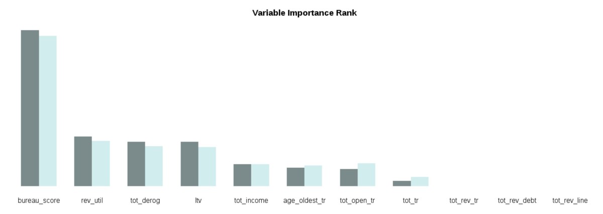
In the YAGeR project (https://github.com/statcompute/yager), two functions have been added with the purpose to assess the variable importance in a GRNN. While the grnn.x_imp() function (https://github.com/statcompute/yager/blob/master/code/grnn.x_imp.R) will provide the importance assessment of a single variable, the grnn.imp() function (https://github.com/statcompute/yager/blob/master/code/grnn.imp.R) can give us a full picture of the variable importance for all variables in the GRNN. The returned value “imp1” is calculated as the decrease in AUC with all values for the variable of interest equal to its mean and the “imp2” is calculated as the decrease in AUC with the variable of interest dropped completely. The variable with a higher value of the decrease in AUC is deemed more important.

Below is an example demonstrating how to assess the variable importance in a GRNN. As shown in the output, there are three variables making no contribution to AUC statistic. It is also noted that dropping three unimportant variables in the GRNN can actually increase AUC in the hold-out sample. What’s more, marginal effects of variables remaining in the GRNN make more sense now with all showing nice monotonic relationships, in particular “tot_open_tr”.

	Y <- df$bad
	X <- scale(df_woe$df[, -1])
	set.seed(2019)
	i <- sample(seq(length(Y)), length(Y) / 4)
	Y1 <- Y[i]
	Y2 <- Y[-i]
	X1 <- X[i, ]
	X2 <- X[-i, ]
	net1 <- grnn.fit(x = X1, y = Y1)
	rst <- grnn.optmiz_auc(net1, lower = 1, upper = 3)
	net2 <- grnn.fit(x = X1, y = Y1, sigma = rst$sigma)
	xrank <- grnn.imp(net2)
	#idx var imp1 imp2
	# 9 woe.bureau_score 0.03629427 0.03490435
	# 8 woe.rev_util 0.01150345 0.01045408
	# 1 woe.tot_derog 0.01033528 0.00925820
	# 10 woe.ltv 0.01033330 0.00910178
	# 11 woe.tot_income 0.00506666 0.00509438
	# 3 woe.age_oldest_tr 0.00430835 0.00476373
	# 4 woe.tot_open_tr 0.00392424 0.00523496
	# 2 woe.tot_tr 0.00123152 0.00215021
	# 5 woe.tot_rev_tr 0.00000000 0.00000000
	# 6 woe.tot_rev_debt 0.00000000 0.00000000
	# 7 woe.tot_rev_line 0.00000000 0.00000000
	excol <- xrank[xrank$imp1 == 0, ]$idx
	#[1] 5 6 7
	MLmetrics::AUC(y_pred = grnn.parpred(net2, X2), y_true = Y2)
	# [1] 0.7584476
	MLmetrics::AUC(y_pred = grnn.parpred(grnn.fit(x = X1[, -excol], y = Y1, sigma = net2$sigma), X2[, -excol]), y_true = Y2)
	# [1] 0.7626386
	barplot(t(as.matrix(xrank[, 3:4])), beside = TRUE, col = c("lightcyan4", "lightcyan2"), border = NA, yaxt = "n",
	names.arg = substring(xrank$var, 5), main = "Variable Importance Rank", cex.names = 1)

view raw

grnn.imp.R

hosted with ❤ by GitHub

Hyper-Parameter Optimization of General Regression Neural Networks

A major advantage of General Regression Neural Networks (GRNN) over other types of neural networks is that there is only a single hyper-parameter, namely the sigma. In the previous post (https://statcompute.wordpress.com/2019/07/06/latin-hypercube-sampling-in-hyper-parameter-optimization), I’ve shown how to use the random search strategy to find a close-to-optimal value of the sigma by using various random number generators, including uniform random, Sobol sequence, and Latin hypercube sampling.

In addition to the random search, we can also directly optimize the sigma based on a pre-defined objective function by using the grnn.optmiz_auc() function (https://github.com/statcompute/yager/blob/master/code/grnn.optmiz_auc.R), in which either Golden section search by default or Brent’s method is employed in the one-dimension optimization. In the example below, the optimized sigma is able to yield a slightly higher AUC in both training and hold-out samples. As shown in the plot, the optimized sigma in red is right next to the best sigma in the random search.

	df <- readRDS("df.rds")
	source("mob.R")
	source("grnnet.R")
	bin_out <- batch_bin(df, 3)
	df_woe <- batch_woe(df, bin_out$BinLst)
	Y <- df$bad
	X <- scale(df_woe$df[, -1])
	set.seed(2019)
	i <- sample(seq(length(Y)), length(Y) / 4)
	Y1 <- Y[i]
	Y2 <- Y[-i]
	X1 <- X[i, ]
	X2 <- X[-i, ]
	net1 <- grnn.fit(x = X1, y = Y1)
	rst1 <- grnn.optmiz_auc(net1, lower = 1, upper = 3, nfolds = 3)
	# sigma auc
	# 2.267056 0.7610545
	S <- gen_latin(min = 1, max = 3, n = 20)
	rst2 <- grnn.search_auc(net1, sigmas = S, nfolds = 3)
	# sigma auc
	# 2.249354 0.7609994
	MLmetrics::AUC(y_pred = grnn.predict(grnn.fit(x = X1, y = Y1, sigma = rst1$sigma), X2), y_true = Y2)
	# 0.7458775
	MLmetrics::AUC(y_pred = grnn.predict(grnn.fit(x = X1, y = Y1, sigma = rst2$best$sigma), X2), y_true = Y2)
	# 0.7458687

view raw

grnn.optmiz_auc.R

hosted with ❤ by GitHub

Modeling Practices of Operational Losses in CCAR

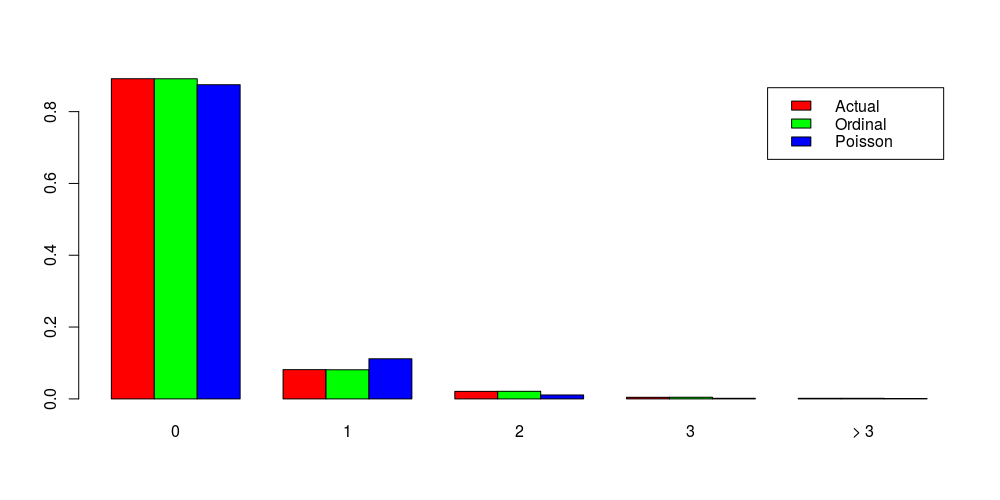
Based upon the CCAR2019 benchmark report published by O.R.X, 88% participants in the survey that submitted results to the Fed used regression models to project operational losses, demonstrating a strong convergence. As described in the report, the OLS regression under the Gaussian distribution still seems the most prevalent approach.

Below is the summary of modeling approaches for operational losses based on my own experience and knowledge that might be helpful for other banking practitioners in CCAR.

	Modeling Frequency
	|
	|– Equi-Dispersion (Baseline)
	| |
	| `– Standard Poisson
	|
	|– Over-Dispersion
	| |
	| |– Negative Binomial
	| |
	| |– Zero-Inflated Poisson
	| |
	| `– Finite Mixture Poisson
	|
	`– Over- or Under-Dispersion
	|
	|– Quasi-Poisson
	|
	|– Hurdle Poisson
	|
	|– Generalized Poisson
	|
	|– Double Poisson
	|
	|– Conway-Maxwell Poisson
	|
	`– Hyper-Poisson

view raw

FrequencyModels

hosted with ❤ by GitHub

	Modeling Loss / Average Loss
	|
	|– Loss without Zeroes
	| |
	| |– Gamma
	| |
	| `– Inverse Gaussian
	|
	|– Loss with Some Zeros
	| |
	| |– Intercept-only ZAGA (Zero-Adjusted Gamma)
	| |
	| |– Intercept-only ZAIG (Zero-Adjusted Inverse Gaussian)
	| |
	| `– Tweedie
	|
	|– Loss with Many Zeros
	| |
	| |– ZAGA (Zero-Adjusted Gamma)
	| |
	| `– ZAIG (Zero-Adjusted Inverse Gaussian)
	|
	`– Loss with Nonzero Threshold Xm
	|
	|– Tobit
	|
	|– Pareto
	|
	`– Shifted Response with Y' = Y – Xm or Y' = Ln(Y / Xm)

view raw

LossModels

hosted with ❤ by GitHub

Develop Performance Benchmark with GRNN

It has been mentioned in https://github.com/statcompute/GRnnet that GRNN is an ideal approach employed to develop performance benchmarks for a variety of risk models. People might wonder what the purpose of performance benchmarks is and why we would even need one at all. Sometimes, a model developer had to answer questions about how well the model would perform even before completing the model. Likewise, a model validator also wondered whether the model being validated has a reasonable performance given the data used and the effort spent. As a result, the performance benchmark, which could be built with the same data sample but an alternative methodology, is called for to address aforementioned questions.

While the performance benchmark can take various forms, including but not limited to business expectations, industry practices, or vendor products, a model-based approach should possess following characteristics:

– Quick prototype with reasonable efforts
– Comparable baseline with acceptable outcomes
– Flexible framework without strict assumptions
– Practical application to broad domains

With both empirical and conceptual advantages, GRNN is able to accommodate each of above-mentioned requirements and thus can be considered an appropriate candidate that might potentially be employed to develop performance benchmarks for a wide variety of models.

Below is an example illustrating how to use GRNN to develop a benchmark model for the logistic regression shown in https://statcompute.wordpress.com/2019/05/04/why-use-weight-of-evidence/. The function grnn.margin() was also employed to explore the marginal effect of each attribute in a GRNN.

	df <- readRDS("df.rds")
	source("mob.R")
	source("grnnet.R")
	# PRE-PROCESS THE DATA WITH MOB PACKAGE
	bin_out <- batch_bin(df, 3)
	bin_out$BinSum[order(-bin_out$BinSum$iv), ]
	# var nbin unique miss min median max ks iv
	# bureau_score 34 315 315 443 692.5 848 35.2651 0.8357
	# tot_rev_line 20 3617 477 0 10573.0 205395 26.8943 0.4442
	# age_oldest_tr 25 460 216 1 137.0 588 20.3646 0.2714
	# tot_derog 7 29 213 0 0.0 32 20.0442 0.2599
	# ltv 17 145 1 0 100.0 176 16.8807 0.1911
	# rev_util 12 101 0 0 30.0 100 16.9615 0.1635
	# tot_tr 15 67 213 0 16.0 77 17.3002 0.1425
	# tot_rev_debt 8 3880 477 0 3009.5 96260 8.8722 0.0847
	# tot_rev_tr 4 21 636 0 3.0 24 9.0779 0.0789
	# tot_income 17 1639 5 0 3400.0 8147167 10.3386 0.0775
	# tot_open_tr 7 26 1416 0 5.0 26 6.8695 0.0282
	# PERFORMAN WOE TRANSFORMATIONS
	df_woe <- batch_woe(df, bin_out$BinLst)
	# PROCESS AND STANDARDIZE THE DATA WITH ZERO MEAN AND UNITY VARIANCE
	Y <- df$bad
	X <- scale(df_woe$df[, -1])
	Reduce(rbind, Map(function(c) data.frame(var = colnames(X)[c], mean = mean(X[, c]), variance = var(X[, c])), seq(dim(X)[2])))
	# var mean variance
	#1 woe.tot_derog 2.234331e-16 1
	#2 woe.tot_tr -2.439238e-15 1
	#3 woe.age_oldest_tr -2.502177e-15 1
	#4 woe.tot_open_tr -2.088444e-16 1
	#5 woe.tot_rev_tr -4.930136e-15 1
	#6 woe.tot_rev_debt -2.174607e-16 1
	#7 woe.tot_rev_line -8.589630e-16 1
	#8 woe.rev_util -8.649849e-15 1
	#9 woe.bureau_score 1.439904e-15 1
	#10 woe.ltv 3.723332e-15 1
	#11 woe.tot_income 5.559240e-16 1
	# INITIATE A GRNN OBJECT
	net1 <- grnn.fit(x = X, y = Y)
	# CROSS-VALIDATION TO CHOOSE THE OPTIONAL SMOOTH PARAMETER
	S <- gen_sobol(min = 0.5, max = 1.5, n = 10, seed = 2019)
	cv <- grnn.cv_auc(net = net1, sigmas = S, nfolds = 5)
	# $test
	# sigma auc
	#1 1.4066449 0.7543912
	#2 0.6205723 0.7303415
	#3 1.0710133 0.7553075
	#4 0.6764866 0.7378430
	#5 1.1322939 0.7553664
	#6 0.8402438 0.7507192
	#7 1.3590402 0.7546164
	#8 1.3031974 0.7548670
	#9 0.7555905 0.7455457
	#10 1.2174429 0.7552097
	# $best
	# sigma auc
	#5 1.132294 0.7553664
	# REFIT A GRNN WITH THE OPTIMAL PARAMETER VALUE
	net2 <- grnn.fit(x = X, y = Y, sigma = cv$best$sigma)
	net2.pred <- grnn.parpred(net2, X)
	# BENCHMARK MODEL PERFORMANCE
	MLmetrics::KS_Stat(y_pred = net2.pred, y_true = df$bad)
	# 44.00242
	MLmetrics::AUC(y_pred = net2.pred, y_true = df$bad)
	# 0.7895033
	# LOGISTIC REGRESSION PERFORMANCE
	MLmetrics::KS_Stat(y_pred = fitted(mdl2), y_true = df$bad)
	# 42.61731
	MLmetrics::AUC(y_pred = fitted(mdl2), y_true = df$bad)
	# 0.7751298
	# MARGINAL EFFECT OF EACH ATTRIBUTE
	par(mfrow = c(3, 4))
	lapply(1:11, function(i) grnn.margin(net2, i))

view raw

use_grnn.R

hosted with ❤ by GitHub

Dummy Is As Dummy Does

In the 1975 edition of “Applied multiple regression/correlation analysis for the behavioral sciences” by Jacob Cohen, an interesting approach of handling missing values in numeric variables was proposed with the purpose to improve the traditional single-value imputation, as described below:

– First of all, impute missing values by the value of mean or median
– And then create a dummy variable to flag out imputed values

In the setting of a regression model, both imputed and dummy variables would be included and therefore the number of independent variables are doubled.

Although the aforementioned approach has long been criticized and eventually abandoned by Cohen himself in the recent edition of the book, I was told that this obsolete technique is still being actively used.

Out of my own curiosity, I applied this dummy imputation approach to the data used in https://statcompute.wordpress.com/2019/05/04/why-use-weight-of-evidence and then compared it with the WoE imputation in the context of Logistic Regression.

Below are my observations:

– Since the dummy approach converts each numeric variable with missing values, the final model tends to have more independent variables, which is not desirable in terms of the model parsimony. For instance, there are 7 independent variables in the model with dummy imputation and only 5 in the model with WoE approach.

– The model performance doesn’t seem to justify the use of more independent variables in the regression with the dummy imputation. As shown in the output below, ROC statistic from the model with WoE approach is significantly better than the one with the dummy imputation based on the DeLong’s test, which is also consistent with the result of Vuong test.

	df <- readRDS("df.rds")
	source("mob.R")
	bin_out <- batch_bin(df, 3)
	bin_out$BinSum[order(-bin_out$BinSum$iv), ]
	# var nbin unique miss min median max ks iv
	# bureau_score 34 315 315 443 692.5 848 35.2651 0.8357
	# tot_rev_line 20 3617 477 0 10573.0 205395 26.8943 0.4442
	# age_oldest_tr 25 460 216 1 137.0 588 20.3646 0.2714
	# tot_derog 7 29 213 0 0.0 32 20.0442 0.2599
	# ltv 17 145 1 0 100.0 176 16.8807 0.1911
	# rev_util 12 101 0 0 30.0 100 16.9615 0.1635
	# tot_tr 15 67 213 0 16.0 77 17.3002 0.1425
	# tot_rev_debt 8 3880 477 0 3009.5 96260 8.8722 0.0847
	# tot_rev_tr 4 21 636 0 3.0 24 9.0779 0.0789
	# tot_income 17 1639 5 0 3400.0 8147167 10.3386 0.0775
	# tot_open_tr 7 26 1416 0 5.0 26 6.8695 0.0282
	# ONLY SELECT VARIABLES WITH IV > 0.1
	dummies <- data.frame(
	bad = df$bad,
	tot_derog = ifelse(is.na(df$tot_derog), mean(df$tot_derog, na.rm = T), df$tot_derog),
	dummy.tot_derog = ifelse(is.na(df$tot_derog), 1, 0),
	tot_tr = ifelse(is.na(df$tot_tr), mean(df$tot_tr, na.rm = T), df$tot_tr),
	dummy.tot_tr = ifelse(is.na(df$tot_tr), 1, 0),
	age_oldest_tr = ifelse(is.na(df$age_oldest_tr), mean(df$age_oldest_tr, na.rm = T), df$age_oldest_tr),
	dummy.age_oldest_tr = ifelse(is.na(df$age_oldest_tr), 1, 0),
	tot_rev_line = ifelse(is.na(df$tot_rev_line), mean(df$tot_rev_line, na.rm = T), df$tot_rev_line),
	dummy.tot_rev_line = ifelse(is.na(df$tot_rev_line), 1, 0),
	rev_util = ifelse(is.na(df$rev_util), mean(df$rev_util, na.rm = T), df$rev_util),
	dummy.rev_util = ifelse(is.na(df$rev_util), 1, 0),
	bureau_score = ifelse(is.na(df$bureau_score), mean(df$bureau_score, na.rm = T), df$bureau_score),
	dummy.bureau_score = ifelse(is.na(df$bureau_score), 1, 0),
	ltv = ifelse(is.na(df$ltv), mean(df$ltv, na.rm = T), df$ltv),
	dummy.ltv = ifelse(is.na(df$ltv), 1, 0))
	dm1 <- summary(glm(bad ~ ., data = dummies, family = "binomial"))
	dx1 <- paste(row.names(dm1$coefficients)[dm1$coefficients[, 4] < 0.05][-1])
	dl1 <- as.formula(paste("bad", paste(dx1, collapse = " + "), sep = " ~ "))
	dm2 <- glm(dl1, data = dummies, family = "binomial")
	# Estimate Std. Error z value Pr(>|z|)
	#(Intercept) 5.827e+00 5.651e-01 10.311 < 2e-16 ***
	#age_oldest_tr -1.595e-03 4.526e-04 -3.523 0.000426 ***
	#tot_rev_line -1.684e-05 2.910e-06 -5.785 7.25e-09 ***
	#dummy.tot_rev_line 5.314e-01 1.434e-01 3.707 0.000210 ***
	#rev_util 3.183e-03 1.171e-03 2.718 0.006574 **
	#bureau_score -1.390e-02 8.075e-04 -17.209 < 2e-16 ***
	#dummy.bureau_score 7.339e-01 1.518e-01 4.835 1.33e-06 ***
	#ltv 2.451e-02 2.249e-03 10.895 < 2e-16 ***
	roc1 <- pROC::roc(response = df$bad, predictor = fitted(mdl2))
	roc2 <- pROC::roc(response = df$bad, predictor = fitted(dm2))
	pROC::roc.test(roc1, roc2, method = "delong", paired = T)
	# DeLong's test for two correlated ROC curves
	# data: roc1 and roc2
	# Z = 4.2369, p-value = 2.266e-05
	# alternative hypothesis: true difference in AUC is not equal to 0
	# sample estimates:
	# AUC of roc1 AUC of roc2
	# 0.7751298 0.7679757
	pscl::vuong(mdl2, dm2)
	# Vuong Non-Nested Hypothesis Test-Statistic:
	# Vuong z-statistic H_A p-value
	# Raw 4.275484 model1 > model2 9.5361e-06
	# AIC-corrected 4.565833 model1 > model2 2.4876e-06
	# BIC-corrected 5.534434 model1 > model2 1.5612e-08

view raw

dummies.R

hosted with ❤ by GitHub

Improve GRNN Efficiency by Weighting

In the post (https://statcompute.wordpress.com/2019/07/14/yet-another-r-package-for-general-regression-neural-network), several advantages of General Regression Neural Network (GRNN) have been discussed. However, as pointed out by Specht, a major weakness of GRNN is the high computational cost required for a GRNN to generate predicted values based on a new input matrix due to its unique network structure, e.g. the number of neurons equal to the number of training samples.

For practical purposes, there is however no need to assign a neuron to each training sample, given the data duplication in real-world model development samples. Instead, a weighting scheme can be employed to reflect the frequency count of each unique training sample. A major benefit of the weight assignment is the ability to improve the efficiency of calculating predicted values, which depends on the extent of data duplicates. More attractively, the weighting application can bring up the possibility of using clustering or binning techniques to preprocess the training data so as to overcome the aforementioned weakness to a large degree.

Below is a demonstration showing the efficiency gain by using the weighting scheme in GRNN.

1. First of all, I constructed a sample data with duplicates to double the size of the original Boston dataset. Based on the constructed data, a GRNN named “N1” was trained.
2. Secondly, I generated another sample data by aggregating the above constructed data based on unique samples and calculating the weight of each unique data point based on its frequency. Based on the aggregated data, another GRNN named “N2” was also trained.

As shown in the output, predicted vectors from both “N1” and “N2” are identical. However, the computing time can be reduced to half by applying the weighting. All R functions used in the example can be found in https://github.com/statcompute/GRnnet/blob/master/code/grnnet.R.

For people interested in the SAS implementation of GRNN, two SAS macros are also available in https://github.com/statcompute/GRnnet/blob/master/code/grnn_learn.SAS and https://github.com/statcompute/GRnnet/blob/master/code/grnn_pred.SAS.

	data(Boston, package = "MASS")
	### CONSTRUCT THE UNWEIGHTED DATA.FRAME WITH DUPLICATES
	df1 <- rbind(Boston[rep(seq(100), 5), ], Boston)
	nrow(df1)
	# 1006
	X1 <- scale(df1[, 1:13])
	Y1 <- df1[, 14]
	N1 <- grnn.fit(X1, Y1)
	### CONSTRUCT THE WEIGHTED DATA.FRAME WITHOUT DUPLICATES
	XY <- data.frame(X1, Y1)
	df2 <- Reduce(rbind, lapply(split(XY, XY[, colnames(XY)], drop = T),
	function(x_) data.frame(x_[1, ], cnt = nrow(x_))))
	nrow(df2)
	# 506
	sum(df2$cnt)
	# 1006
	X2 <- as.matrix(df2[, 1:13])
	Y2 <- df2[, 14]
	W2 <- df2[, 15]
	N2 <- grnn.fit(X2, Y2, W2)
	### IDENTICAL PREDICTED VALUES WITH UNWEIGHTED AND WEIGHTED DATA.FRAMES
	grnn.predone(N1, X1[1, ])
	# 24.69219
	grnn.predone(N2, X1[1, ])
	# 24.69219
	all.equal(grnn.predict(N1, X1[1:100, ]), grnn.predict(N2, X1[1:100, ]))
	# TRUE
	### COMPUTING TIME ROUGHLY LINEAR WITH RESPECT TO SIZE OF UNIQUE TRAINING SAMPLE
	rbenchmark::benchmark(replications = 10, order = "elapsed", relative = "elapsed",
	columns = c("test", "replications", "elapsed", "relative"),
	" NO WEIGHT" = grnn.predict(N1, X1[1:100, ]),
	"USE WEIGHT" = grnn.predict(N2, X1[1:100, ])
	)
	# test replications elapsed relative
	# 2 USE WEIGHT 10 2.157 1.000
	# 1 NO WEIGHT 10 5.506 2.553

view raw

wt_grnn.R

hosted with ❤ by GitHub

Yet Another R Package for General Regression Neural Network

Compared with other types of neural networks, General Regression Neural Network (Specht, 1991) is advantageous in several aspects.

1. Being an universal approximation function, GRNN has only one tuning parameter to control the overall generalization
2. The network structure of GRNN is surprisingly simple, with only one hidden layer and the number of neurons equal to the number of training samples.
3. GRNN is always able to converge globally and won’t be trapped by local solutions.
4. The training of GRNN is a simple 1-pass, regardless of the sample size, and doesn’t require time-consuming iterations.
5. Since any projected value of GRNN is the weighted average of training samples, predictions are bounded by the observed range.

The grnn package (https://cran.r-project.org/web/packages/grnn/index.html), which has not been updated since 2013, is the only implementation of GRNN on CRAN and was designed elegantly with a parsimonious set of functions and lots of opportunities for potential improvements.

The YAGeR project (https://github.com/statcompute/yager) is my attempt to provide a R implementation of GRNN, with several enhancements.

1. While the training function grnn.fit() is very similar to learn() and smooth() in the grnn package. three functions were designed to provide GRNN projections. The grnn.predone() function generates one projected value based on an input vector. Both grnn.predict() and grnn.parpred() functions generate a vector of projected values based on an input matrix. The only difference is that grnn.parpred() runs in parallel and therefore can be 3 times faster than grnn.predict() on my 4-core workstation.
2. While tuning the only hyper-parameter is the key in GRNN training, there are two functions in the GRnnet project to search for the optimal parameter through the n-fold cross validation, including grnn.cv_r2() for numeric outcomes and grnn.cv_auc() for binary outcomes.
3. In grnn.predone() function, while the default projection is based on the Euclidean distance, there is an option to calculate the GRNN projection based on the Manhattan distance as well for the sake of computational simplicity (Specht, 1991).

In the banking industry, GRNN can be useful in several areas. First of all, it can be employed as the replacement of splines to approximate the term structure of interest rates. Secondly, like other neural networks, it can be used in Fraud Detection and Anti-Money Laundering given its flexibility. At last, in the credit risk modeling, it can also be used to develop performance benchmarks and rapid prototypes for scorecards or Expected Loss models due to the simplicity.

Monotonic Binning Driven by Decision Tree

After the development of MOB package (https://github.com/statcompute/MonotonicBinning), I was asked by a couple users about the possibility of using the decision tree to drive the monotonic binning. Although I am not aware of any R package implementing the decision tree with the monotonic constraint, I did manage to find a solution based upon the decision tree.

The Rborist package is an implementation of the Random Forest that would enforce the monotonicity at the local level within each tree but not at the global level for the whole forest. However, with a few tweaks on the Rborist syntax, it is not difficult to convert the forest with many trees into the forest with a single tree. After all necessary adjustments, I finally ended up with a decision tree that can be used to drive the monotonic binning algorithm, as shown in the arb_bin() function below, and will consider adding it into the MOB package later.

	arb_bin <- function(data, y, x) {
	yname <- deparse(substitute(y))
	xname <- deparse(substitute(x))
	df1 <- subset(data, !is.na(data[[xname]]) & data[[yname]] %in% c(0, 1), select = c(xname, yname))
	df2 <- data.frame(y = df1[[yname]], x = df1[[xname]])
	spc <- cor(df2[, 2], df2[, 1], method = "spearman", use = "complete.obs")
	mdl <- Rborist::Rborist(as.matrix(df2$x), df2$y, noValidate = T, nTree = 1, regMono = spc / abs(spc),
	ctgCensus = "prob", minInfo = exp(-100), nSamp = nrow(df2) , withRepl = F)
	df3 <- data.frame(y = df2$y, x = df2$x, yhat = predict(mdl, newdata = as.matrix(df2$x), ctgCensus = "prob")$yPred)
	df4 <- Reduce(rbind,
	lapply(split(df3, df3$yhat),
	function(x) data.frame(maxx = max(x$x), yavg = mean(x$y), yhat = round(mean(x$yhat), 8))))
	df5 <- df4[order(df4$maxx), ]
	h <- ifelse(df5[["yavg"]][1] %in% c(0, 1), 2, 1)
	t <- ifelse(df5[["yavg"]][nrow(df5)] %in% c(0, 1), 2, 1)
	cuts <- df5$maxx[h:max(h, (nrow(df5) – t))]
	return(list(df = manual_bin(data, yname, xname, cuts = cuts),
	cuts = cuts))
	}
	arb_bin(df, bad, rev_util)
	# bin rule freq dist mv_cnt bad_freq bad_rate woe iv ks
	# 01 $X <= 24 2653 0.4545 0 414 0.1560 -0.3320 0.0452 13.6285
	# 02 $X > 24 & $X <= 36 597 0.1023 0 96 0.1608 -0.2963 0.0082 16.3969
	# 03 $X > 36 & $X <= 40 182 0.0312 0 32 0.1758 -0.1890 0.0011 16.9533
	# 04 $X > 40 & $X <= 58 669 0.1146 0 137 0.2048 -0.0007 0.0000 16.9615
	# 05 $X > 58 & $X <= 60 77 0.0132 0 16 0.2078 0.0177 0.0000 16.9381
	# 06 $X > 60 & $X <= 72 408 0.0699 0 95 0.2328 0.1636 0.0020 15.7392
	# 07 $X > 72 & $X <= 73 34 0.0058 0 8 0.2353 0.1773 0.0002 15.6305
	# 08 $X > 73 & $X <= 75 62 0.0106 0 16 0.2581 0.2999 0.0010 15.2839
	# 09 $X > 75 & $X <= 83 246 0.0421 0 70 0.2846 0.4340 0.0089 13.2233
	# 10 $X > 83 & $X <= 96 376 0.0644 0 116 0.3085 0.5489 0.0225 9.1266
	# 11 $X > 96 & $X <= 98 50 0.0086 0 17 0.3400 0.6927 0.0049 8.4162
	# 12 $X > 98 483 0.0827 0 179 0.3706 0.8263 0.0695 0.0000
	arb_bin(df, bad, tot_derog)
	# bin rule freq dist mv_cnt bad_freq bad_rate woe iv ks
	# 00 is.na($X) 213 0.0365 213 70 0.3286 0.6416 0.0178 2.7716
	# 01 $X <= 0 2850 0.4883 0 367 0.1288 -0.5559 0.1268 20.0442
	# 02 $X > 0 & $X <= 1 891 0.1526 0 193 0.2166 0.0704 0.0008 18.9469
	# 03 $X > 1 & $X <= 2 478 0.0819 0 121 0.2531 0.2740 0.0066 16.5222
	# 04 $X > 2 & $X <= 3 332 0.0569 0 86 0.2590 0.3050 0.0058 14.6321
	# 05 $X > 3 & $X <= 23 1064 0.1823 0 353 0.3318 0.6557 0.0931 0.4370
	# 06 $X > 23 9 0.0015 0 6 0.6667 2.0491 0.0090 0.0000

view raw

do_arb_bin.R

hosted with ❤ by GitHub

Chunk Averaging of GLM

Chunk Average (CA) is an interesting concept proposed by Matloff in the chapter 13 of his book “Parallel Computing for Data Science”. The basic idea is to partition the entire model estimation sample into chunks and then to estimate a glm for each chunk. Under the i.i.d assumption, the CA estimator with the chunked data is asymptotically equivalent to the estimator with the full data. The possibility of converting the full model estimation with an excessively large dataset to the chunked estimation with small pieces is particularly attractive in real-world model developments where the model convergence could be challenging given the data size.

The ca_glm() function below is my attempt to implement the Chunk Averaging of GLM. As shown, CA estimations by various chunks are consistent with the estimation with the full data.

	df1 <- read.csv("/mnt/d/projects/data/credit_count.txt")
	df2 <- df1[which(df1$CARDHLDR == 1), ]
	ca_glm <- function(fml, data, family, nchunk) {
	cls <- parallel::makeCluster(nchunk, type = "PSOCK")
	df1 <- parallel::parLapplyLB(cls, parallel::clusterSplit(cls, seq(nrow(data))),
	function(c_) data[c_,])
	parallel::clusterExport(cls, c("fml", "family", "data"), envir = environment())
	est <- parallel::parLapplyLB(cls, df1,
	function(d_) cbind(coef(summary(glm(fml, data = d_, family = family)))[, 1:2], nrow(d_) / nrow(data)))
	parallel::stopCluster(cls)
	df2 <- Reduce(rbind,
	lapply(est,
	function(e_) data.frame(name = format(rownames(e_), justify = "left"),
	beta = e_[, 1] * e_[, 3],
	var = (e_[, 2] * e_[, 3])^ 2)))
	df3 <- Reduce(rbind,
	lapply(split(df2, df2$name),
	function(d_) data.frame(name = d_$name[1],
	beta = sum(d_$beta),
	stder = sum(d_$var) ^ 0.5)))
	return(cbind(df3, zvalue = df3$beta / df3$stder, pvalue = 2 * pnorm(-abs(df3$beta / df3$stder))))
	}
	y <- "DEFAULT"
	x <- c("MAJORDRG", "MINORDRG", "INCOME")
	f <- as.formula(paste(y, paste(x, collapse = " + "), sep = " ~ "))
	summary(glm(f, data = df2, family = "binomial"))$coef
	# Estimate Std. Error z value Pr(|z|)
	# (Intercept) -1.2215970658 9.076358e-02 -13.459110 2.721743e-41
	# MAJORDRG 0.2030503715 6.921101e-02 2.933787 3.348538e-03
	# MINORDRG 0.1919770456 4.783751e-02 4.013107 5.992472e-05
	# INCOME -0.0004705599 3.918955e-05 -12.007282 3.253645e-33
	ca_glm(f, df2, "binomial", 2)[rank(rownames(summary(glm(f, data = df2, family = "binomial"))$coef)), ]
	# name beta stder zvalue pvalue
	# (Intercept) -1.2001768403 9.161584e-02 -13.100102 3.288167e-39
	# MAJORDRG 0.2024462446 6.936634e-02 2.918508 3.517103e-03
	# MINORDRG 0.1928945270 4.799079e-02 4.019407 5.834476e-05
	# INCOME -0.0004811946 3.974214e-05 -12.107919 9.589651e-34
	ca_glm(f, df2, "binomial", 4)[rank(rownames(summary(glm(f, data = df2, family = "binomial"))$coef)), ]
	# name beta stder zvalue pvalue
	# (Intercept) -1.1891569565 9.257056e-02 -12.845952 9.063064e-38
	# MAJORDRG 0.2008495039 7.084338e-02 2.835120 4.580846e-03
	# MINORDRG 0.2075713235 4.883860e-02 4.250149 2.136283e-05
	# INCOME -0.0004902169 4.032866e-05 -12.155548 5.360122e-34
	y <- "MAJORDRG"
	x <- c("ADEPCNT", "MINORDRG", "INCPER")
	f <- as.formula(paste(y, paste(x, collapse = " + "), sep = " ~ "))
	summary(glm(f, data = df2, family = "poisson"))$coef
	# Estimate Std. Error z value Pr(|z|)
	# (Intercept) -2.875143e+00 6.565395e-02 -43.792384 0.000000e+00
	# ADEPCNT 2.091082e-01 2.137937e-02 9.780844 1.360717e-22
	# MINORDRG 5.249111e-01 1.775197e-02 29.569171 3.723779e-192
	# INCPER 2.018335e-05 1.683187e-06 11.991151 3.953735e-33
	ca_glm(f, df2, "poisson", 2)[rank(rownames(summary(glm(f, data = df2, family = "poisson"))$coef)), ]
	# name beta stder zvalue pvalue
	# (Intercept) -2.876932e+00 6.589413e-02 -43.659914 0.000000e+00
	# ADEPCNT 2.072821e-01 2.151670e-02 9.633546 5.770316e-22
	# MINORDRG 5.269996e-01 1.791464e-02 29.417248 3.304900e-190
	# INCPER 2.015435e-05 1.692556e-06 11.907644 1.079855e-32
	ca_glm(f, df2, "poisson", 4)[rank(rownames(summary(glm(f, data = df2, family = "poisson"))$coef)), ]
	# name beta stder zvalue pvalue
	# (Intercept) -2.890965e+00 6.723771e-02 -42.996187 0.000000e+00
	# ADEPCNT 2.112105e-01 2.179890e-02 9.689044 3.356557e-22
	# MINORDRG 5.334541e-01 1.848846e-02 28.853359 4.598288e-183
	# INCPER 2.012836e-05 1.744654e-06 11.537165 8.570364e-31

view raw

ca_glm.R

hosted with ❤ by GitHub

Latin Hypercube Sampling in Hyper-Parameter Optimization

In my previous post https://statcompute.wordpress.com/2019/02/03/sobol-sequence-vs-uniform-random-in-hyper-parameter-optimization/, I’ve shown the difference between the uniform pseudo random and the quasi random number generators in the hyper-parameter optimization of machine learning.

Latin Hypercube Sampling (LHS) is another interesting way to generate near-random sequences with a very simple idea. Let’s assume that we’d like to perform LHS for 10 data points in the 1-dimension data space. We first partition the whole data space into 10 equal intervals and then randomly select a data point from each interval. For the N-dimension LHS with N > 1, we just need to independently repeat the 1-dimension LHS for N times and then randomly combine these sequences into a list of N-tuples.

LHS is similar to the Uniform Random in the sense that the Uniform Random number is drawn within each equal-space interval. On the other hand, LHS covers the data space more evenly in a way similar to the Quasi Random, such as Sobol Sequence. A comparison below shows how each of three looks like in the 2-dimension data space.

unifm_2d <- function(n, seed) {
  set.seed(seed)
  return(replicate(2, runif(n)))
}

sobol_2d <- function(n, seed) {
  return(randtoolbox::sobol(n, dim = 2, scrambling = 3, seed = seed))
}

latin_2d <- function(n, seed) {
  set.seed(seed)
  return(lhs::randomLHS(n, k = 2))
}

par(mfrow = c(1, 3))
plot(latin_2d(100, 2019), main = "LATIN HYPERCUBE", xlab = '', ylab = '', cex = 2, col = "blue")
plot(sobol_2d(100, 2019), main = " SOBOL SEQUENCE", xlab = '', ylab = '', cex = 2, col = "red")
plot(unifm_2d(100, 2019), main = " UNIFORM RANDOM", xlab = '', ylab = '', cex = 2, col = "black")

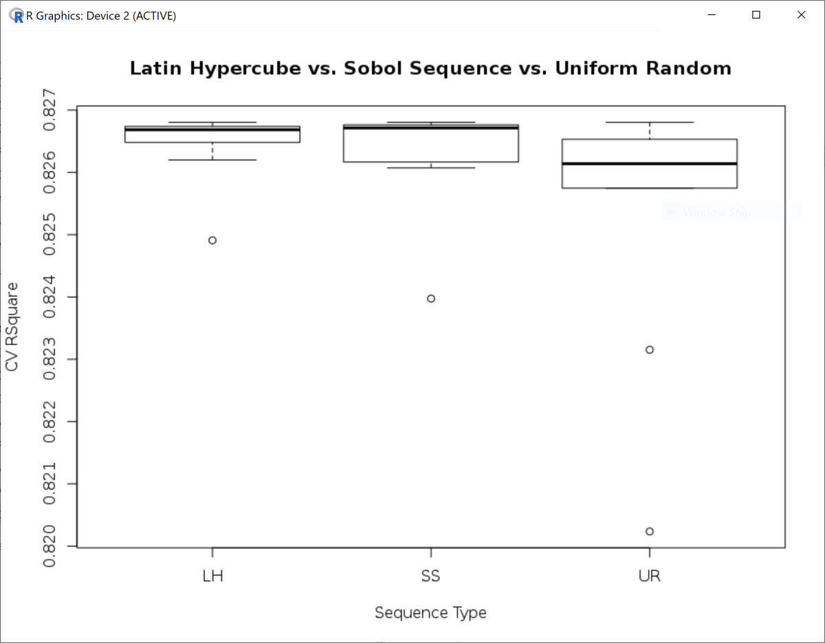
In the example below, three types of random numbers are applied to the hyper-parameter optimization of General Regression Neural Network (GRNN) in the 1-dimension case. While both Latin Hypercube and Sobol Sequence generate similar averages of CV R-squares, the variance of CV R-squares for Latin Hypercube is much lower. With no surprise, the performance of simple Uniform Random remains the lowest, e.g. lower mean and higher variance.

data(Boston, package = "MASS")
df <- data.frame(y = Boston[, 14], scale(Boston[, -14]))
gn <- grnn::smooth(grnn::learn(df), sigma = 1)

grnn.predict <- function(nn, dt) {
  Reduce(c, lapply(seq(nrow(dt)), function(i) grnn::guess(nn, as.matrix(dt[i, ]))))
}

r2 <- function(act, pre) {
  return(1 - sum((pre - act) ^ 2) / sum((act - mean(act)) ^ 2))
}

grnn.cv <- function(nn, sigmas, nfolds, seed = 2019) {
  dt <- nn$set
  set.seed(seed)
  fd <- caret::createFolds(seq(nrow(dt)), k = nfolds)
  cv <- function(s) {
    rs <- Reduce(rbind,
                 lapply(fd,
                        function(f) data.frame(Ya = nn$Ya[unlist(f)],
                                               Yp = grnn.predict(grnn::smooth(grnn::learn(nn$set[unlist(-f), ]), s),
                                                                 nn$set[unlist(f), -1]))))
    return(data.frame(sigma = s, R2 = r2(rs$Ya, rs$Yp)))
  }
  cl <- parallel::makeCluster(min(nfolds, parallel::detectCores() - 1), type = "PSOCK")
  parallel::clusterExport(cl, c("fd", "nn", "grnn.predict", "r2"),  envir = environment())
  rq <- Reduce(rbind, parallel::parLapply(cl, sigmas, cv))
  parallel::stopCluster(cl)
  return(rq[rq$R2 == max(rq$R2), ])
}

gen_unifm <- function(min = 0, max = 1, n, seed) {
  set.seed(seed)
  return(round(min + (max - min) * runif(n), 8))
}

gen_sobol <- function(min = 0, max = 1, n, seed) {
  return(round(min + (max - min) * randtoolbox::sobol(n, dim = 1, scrambling = 3, seed = seed), 8))
}

gen_latin <- function(min = 0, max = 1, n, seed) {
  set.seed(seed)
  return(round(min + (max - min) * c(lhs::randomLHS(n, k = 1)), 8))
}

nfold <- 10
nseed <- 10

sobol_out <- Reduce(rbind, lapply(seq(nseed), function(x) grnn.cv(gn, gen_sobol(0.1, 1, 10, x), nfold)))
latin_out <- Reduce(rbind, lapply(seq(nseed), function(x) grnn.cv(gn, gen_latin(0.1, 1, 10, x), nfold)))
unifm_out <- Reduce(rbind, lapply(seq(nseed), function(x) grnn.cv(gn, gen_unifm(0.1, 1, 10, x), nfold)))

out <- rbind(cbind(type = rep("LH", nseed), latin_out),
             cbind(type = rep("SS", nseed), sobol_out),
             cbind(type = rep("UR", nseed), unifm_out))

title <- "Latin Hypercube vs. Sobol Sequence vs. Uniform Random"
boxplot(R2 ~ type, data = out, main = title, ylab = "CV RSquare", xlab = "Sequence Type")

aggregate(R2 ~ type, data = out, function(x) round(c(avg = mean(x), var = var(x)), 8))
#type     R2.avg     R2.var
#  LH 0.82645414 0.00000033
#  SS 0.82632171 0.00000075
#  UR 0.82536693 0.00000432

Parallel R: Socket or Fork

In the R parallel package, there are two implementations of parallelism, e.g. fork and socket, with pros and cons.

For the fork, each parallel thread is a complete duplication of the master process with the shared environment, including objects or variables defined prior to the kickoff of parallel threads. Therefore, it runs fast. However, the major limitation is that the fork doesn’t work on the Windows system.

On the other hand, the socket works on all operating systems. Each thread runs separately without sharing objects or variables, which can only be passed from the master process explicitly. As a result, it runs slower due to the communication overhead.

Below is an example showing the performance difference between the fork and the socket. A self-defined filter function runs in parallel and exacts three rows out of 336,776 that are meeting criteria. As shown, the fork runs 40% faster than the socket.

df <- read.csv("data/nycflights")

ex <- expression(carrier == "UA" & origin == "EWR" & day == 1 & is.na(arr_time))
# SELECT 3 ROWS OUT OF 336,776
#        year month day dep_time dep_delay arr_time arr_delay carrier tailnum flight origin dest air_time ...
# 56866  2013    11   1       NA        NA       NA        NA      UA            252    EWR  IAH       NA ...
# 84148  2013    12   1       NA        NA       NA        NA      UA            643    EWR  ORD       NA ...
# 251405 2013     7   1       NA        NA       NA        NA      UA            394    EWR  ORD       NA ...

parFilter <- function(df, ex, type) {
  cn <- parallel::detectCores() - 1
  cl <- parallel::makeCluster(cn, type = type)
  ### DIVIDE THE DATAFRAME BASED ON # OF CORES
  sp <- parallel::parLapply(cl, parallel::clusterSplit(cl, seq(nrow(df))),
                            function(c_) df[c_,])
  ### PASS THE OBJECT FROM MASTER PROCESS TO EACH NODE
  parallel::clusterExport(cl, "ex")
  ### EXTRACT ROW INDEX ON EACH NODE
  id <- Reduce(c, parallel::parLapply(cl, sp,
                                      function(s_) with(s_, eval(ex))))
  parallel::stopCluster(cl)
  return(df[which(id),])
}

rbenchmark::benchmark(replications = 10, order = "elapsed", relative = "elapsed",
                        columns = c("test", "replications", "elapsed", "relative"),
  "  FORK" = parFilter(df, ex, "FORK"),
  "SOCKET" = parFilter(df, ex, "PSOCK")
)
#     test replications elapsed relative
# 1   FORK           10  59.396    1.000
# 2 SOCKET           10  83.856    1.412

WoE Transformation for Loss Given Default Models

In the intro section of my MOB package (https://github.com/statcompute/MonotonicBinning#introduction), reasons and benefits of using WoE transformations in the context of logistic regressions with binary outcomes had been discussed. What’s more, the similar idea can be easily generalized to other statistical models in the credit risk area, such as LGD (Loss Given Default) models with fractional outcomes.

Measuring the ratio between net and gross charge-offs, LGD can take any value within the unity interval of [0, 1] with no unanimous consensus on the distributional assumption either academically or empirically. In the banking industry, a popular approach to model LGD is the use of Quasi-Binomial models that makes no assumption of any statistical distribution but merely specifies the conditional mean by a Logit link function. With the specification of Logit link, the idea of WoE transformations can be ported directly from logistic regressions to Quasi-Binomial models.

The example below shows how to perform WoE transformations through monotonic binning based upon the fractional outcome, e.g. LGD, by using the function qtl_lgd() (https://github.com/statcompute/MonotonicBinning/blob/master/code/qtl_lgd.R).

	qtl_lgd(df, lgd, ltv)
	#$df
	# bin rule freq dist mv_cnt mean_y woe iv ks
	# 1 01 $X <= 0.2442486803 320 0.1257 0 0.0948 -1.0370 0.0987 9.5173
	# 2 02 $X > 0.2442486803 & $X <= 0.3994659888 318 0.1250 0 0.0994 -0.9850 0.0900 18.6516
	# 3 03 $X > 0.3994659888 & $X <= 0.5314432946 318 0.1250 0 0.1265 -0.7135 0.0515 25.8646
	# 4 04 $X > 0.5314432946 & $X <= 0.6594855396 318 0.1250 0 0.1283 -0.6974 0.0494 32.9504
	# 5 05 $X > 0.6594855396 & $X <= 0.7917383883 318 0.1250 0 0.1769 -0.3182 0.0116 36.5819
	# 6 06 $X > 0.7917383883 & $X <= 0.9243704807 320 0.1257 0 0.2788 0.2683 0.0097 32.9670
	# 7 07 $X > 0.9243704807 & $X <= 1.0800711662 317 0.1246 0 0.4028 0.8251 0.1020 20.6104
	# 8 08 $X > 1.0800711662 316 0.1242 0 0.5204 1.3006 0.2681 0.0000
	# $cuts
	# [1] 0.2442487 0.3994660 0.5314433 0.6594855 0.7917384 0.9243705 1.0800712

view raw

use_qtl_lgd.R

hosted with ❤ by GitHub

As demonstrated in the outcome table, the average LGD increases along with the LTV (Loan-to-Value) and the WoE transformation of LTV is strictly linear with respect to the Logit of average LGD.

Faster Way to Slice Dataframe by Row

When we’d like to slice a dataframe by row, we can employ the split() function or the iter() function in the iterators package.

By leveraging the power of parallelism, I wrote an utility function slice() to faster slice the dataframe. In the example shown below, the slice() is 3 times more efficient than the split() or the iter() to select 2 records out of 5,960 rows.

df <- read.csv("hmeq.csv")

nrow(df)
# [1] 5960

slice <- function(df) {
  return(parallel::mcMap(function(i) df[i, ], seq(nrow(df)), mc.cores = parallel::detectCores()))
}

Reduce(rbind, Filter(function(x) x$DEROG == 10, slice(df)))
#     BAD  LOAN MORTDUE VALUE  REASON   JOB YOJ DEROG DELINQ     CLAGE NINQ CLNO  DEBTINC
#3094   1 16800   16204 27781 HomeImp Other   1    10      0 190.57710    0    9 27.14689
#3280   1 17500   76100 98500 DebtCon Other   5    10      1  59.83333    5   16       NA

rbenchmark::benchmark(replications = 10, order = "elapsed", relative = "elapsed",
                        columns = c("test", "replications", "elapsed", "relative"),
  "SPLIT" = Reduce(rbind, Filter(Negate(function(x) x$DEROG != 10), split(df, seq(nrow(df))))),
  "ITER " = Reduce(rbind, Filter(Negate(function(x) x$DEROG != 10), as.list(iterators::iter(df, by = "row")))),
  "SLICE" = Reduce(rbind, Filter(Negate(function(x) x$DEROG != 10), slice(df)))
)
#  test replications elapsed relative
# SLICE           10   2.224    1.000
# SPLIT           10   7.185    3.231
# ITER            10   7.375    3.316

Granular Weighted Binning by Generalized Boosted Model

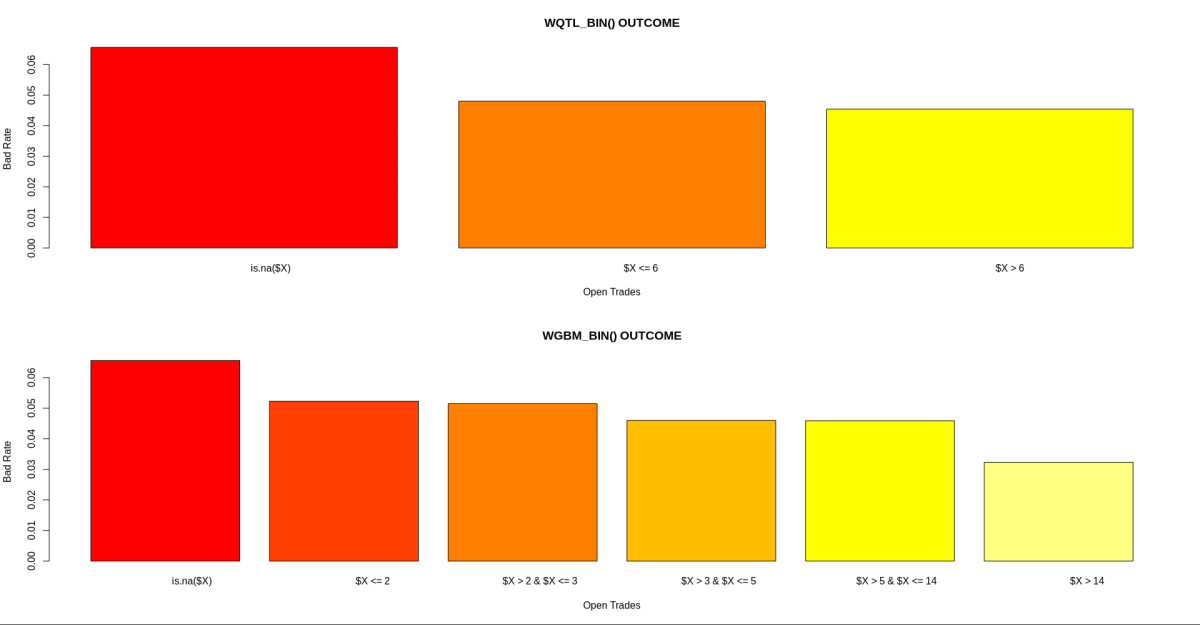
In the post https://statcompute.wordpress.com/2019/04/27/more-general-weighted-binning, I’ve shown how to do the weighted binning with the function wqtl_bin() by the iterative partitioning. However, the outcome from wqtl_bin() sometimes can be too coarse. The function wgbm_bin() (https://github.com/statcompute/MonotonicBinning/blob/master/code/wgbm_bin.R) leverages the idea of gbm() that implements the Generalized Boosted Model and generates more granular weighted binning outcomes.

Below is the demonstration showing the difference between wqtl_bin() and wgbm_bin() outcomes. Even with the same data, the wgbm_bin() function is able to generate a more granular binning result and 14% higher Information Value.

	df <- readRDS("archive/accepts.rds")
	head(df, 1)
	# bankruptcy bad app_id tot_derog tot_tr age_oldest_tr tot_open_tr tot_rev_tr tot_rev_debt tot_rev_line rev_util bureau_score purch_price msrp
	# 0 0 1001 6 7 46 NaN NaN NaN NaN 0 747 19678 17160
	# down_pyt purpose loan_term loan_amt ltv tot_income used_ind weight
	# 947.15 LEASE 36 18730.85 109 4800 0 4.75
	### BY ITERATIVE PARTITION ###
	source("wqtl_bin.R")
	wqtl_bin(df, bad, tot_open_tr, weight)
	# bin rule cnt freq dist mv_wt bad_freq bad_rate woe iv ks
	# 00 is.na($X) 1416 5398.50 0.2323 5398.5 354 0.0656 0.2573 0.0173 6.7157
	# 01 $X <= 6 2994 12050.25 0.5185 0.0 579 0.0480 -0.0722 0.0026 3.0908
	# 02 $X > 6 1427 5792.00 0.2492 0.0 263 0.0454 -0.1315 0.0041 0.0000
	### BY GENERALIZED BOOSTED MODEL ###
	source("wgbm_bin.R")
	wgbm_bin(df, bad, tot_open_tr, weight)
	# bin rule cnt freq dist mv_wt bad_freq bad_rate woe iv ks
	# 00 is.na($X) 1416 5398.50 0.2323 5398.5 354 0.0656 0.2573 0.0173 6.7157
	# 01 $X <= 2 525 2085.00 0.0897 0.0 109 0.0523 0.0166 0.0000 6.8658
	# 02 $X > 2 & $X <= 3 605 2408.75 0.1036 0.0 124 0.0515 0.0004 0.0000 6.8695
	# 03 $X > 3 & $X <= 5 1319 5342.75 0.2299 0.0 246 0.0460 -0.1169 0.0030 4.3181
	# 04 $X > 5 & $X <= 14 1899 7696.50 0.3312 0.0 353 0.0459 -0.1210 0.0046 0.5213
	# 05 $X > 14 73 309.25 0.0133 0.0 10 0.0323 -0.4846 0.0025 0.0000

view raw

use_wtwoe.R

hosted with ❤ by GitHub

Why Use Weight of Evidence?

I had been asked why I spent so much effort on developing SAS macros and R functions to do monotonic binning for the WoE transformation, given the availability of other cutting-edge data mining algorithms that will automatically generate the prediction with whatever predictors fed in the model. Nonetheless, what really distinguishes a good modeler from the rest is how to handle challenging data issues before feeding data in the model, including missing values, outliers, linearity, and predictability, in a scalable way that can be rolled out to hundreds or even thousands of potential model drivers in the production environment.

The WoE transformation through monotonic binning provides a convenient way to address each of aforementioned concerns.

1. Because WoE is a piecewise transformation based on the data discretization, all missing values would fall into a standalone category either by itself or to be combined with the neighbor that shares a similar event probability. As a result, the special treatment for missing values is not necessary.

2. After the monotonic binning of each variable, since the WoE value for each bin is a projection from the predictor into the response that is defined by the log ratio between event and non-event distributions, any raw value of the predictor doesn’t matter anymore and therefore the issue related to outliers would disappear.

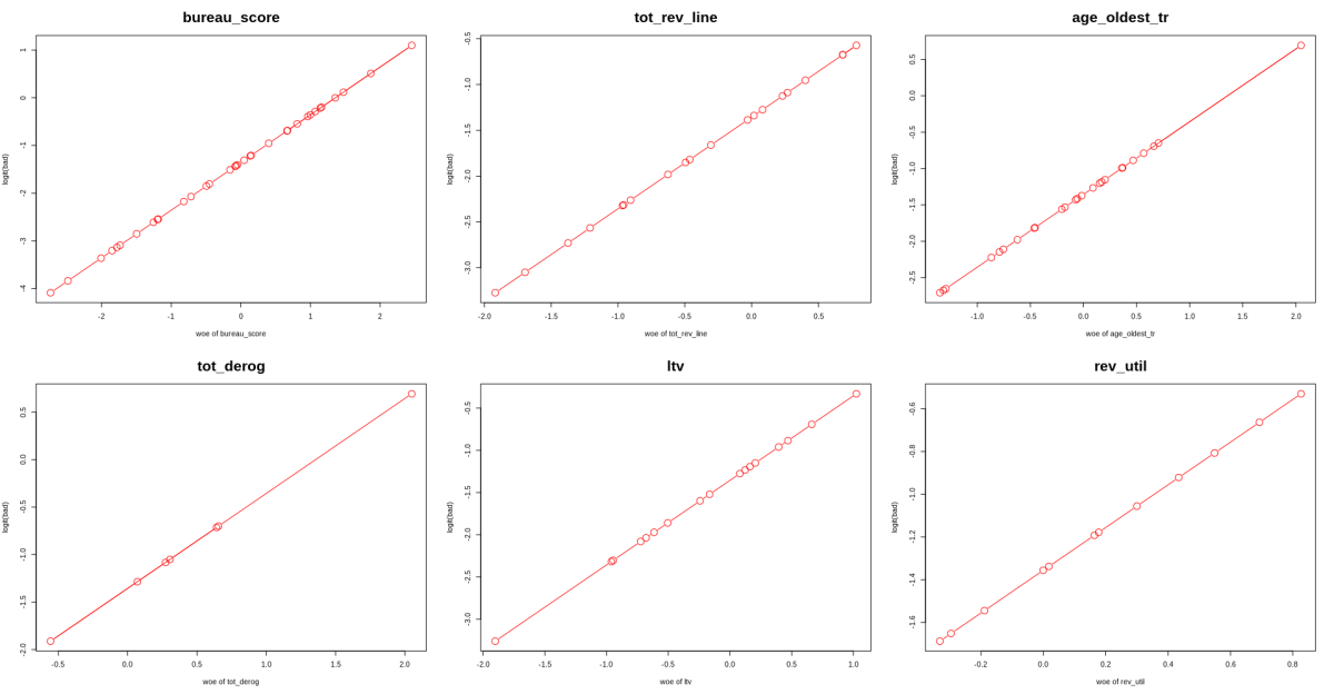
3. While many modelers would like to use log or power transformations to achieve a good linear relationship between the predictor and log odds of the response, which is heuristic at best with no guarantee for the good outcome, the WoE transformation is strictly linear with respect to log odds of the response with the unity correlation. It is also worth mentioning that a numeric variable and its strictly monotone functions should converge to the same monotonic WoE transformation.

4. At last, because the WoE is defined as the log ratio between event and non-event distributions, it is indicative of the separation between cases with Y = 0 and cases with Y = 1. As the weighted sum of WoE values with the weight being the difference in event and non-event distributions, the IV (Information Value) is an important statistic commonly used to measure the predictor importance.

Below is a simple example showing how to use WoE transformations in the estimation of a logistic regression.

	df <- readRDS("df.rds")
	### SHOWING THE RESPONSE IN THE LAST COLUMN ###
	head(df, 2)
	#tot_derog tot_tr age_oldest_tr tot_open_tr tot_rev_tr tot_rev_debt tot_rev_line rev_util bureau_score ltv tot_income bad
	# 6 7 46 NaN NaN NaN NaN 0 747 109 4800.00 0
	# 0 21 153 6 1 97 4637 2 744 97 5833.33 0
	source("mob.R")
	bin_out <- batch_bin(df, 3)
	bin_out$BinSum
	# var nbin unique miss min median max ks iv
	# tot_derog 7 29 213 0 0.0 32 20.0442 0.2599
	# tot_tr 15 67 213 0 16.0 77 17.3002 0.1425
	# ……
	top <- paste(bin_out$BinSum[order(bin_out$BinSum[["iv"]], decreasing = T), ][1:6, "var"], sep = '')
	par(mfrow = c(2, 3))
	lapply(top, function(x) plot(bin_out$BinLst[[x]]$df[["woe"]],
	log(bin_out$BinLst[[x]]$df[["bad_rate"]] / (1 – bin_out$BinLst[[x]]$df[["bad_rate"]])),
	type = "b", main = x, cex.main = 2, xlab = paste("woe of", x), ylab = "logit(bad)", cex = 2, col = "red"))
	df_woe <- batch_woe(df, bin_out$BinLst)
	str(df_woe$df)
	#'data.frame': 5837 obs. of 12 variables:
	# $ idx_ : int 1 2 3 4 5 6 7 8 9 10 …
	# $ woe.tot_derog : num 0.656 -0.556 -0.556 0.274 0.274 …
	# $ woe.tot_tr : num 0.407 -0.322 -0.4 -0.322 0.303 …
	# ……
	### PARSE VARIABLES WITH IV > 0.1 ###
	x1 <- paste("woe", bin_out$BinSum[bin_out$BinSum[["iv"]] > 0.1, ]$var, sep = ".")
	# "woe.tot_derog" "woe.tot_tr" "woe.age_oldest_tr" "woe.tot_rev_line" "woe.rev_util" "woe.bureau_score" "woe.ltv"
	fml1 <- as.formula(paste("bad", paste(x1, collapse = " + "), sep = " ~ "))
	sum1 <- summary(glm(fml1, data = cbind(bad = df$bad, df_woe$df), family = "binomial"))
	### PARSE SIGNIFICANT VARIABLES WITH P-VALUE < 0.05 ###
	x2 <- paste(row.names(sum1$coefficients)[sum1$coefficients[, 4] < 0.05][-1])
	# "woe.age_oldest_tr" "woe.tot_rev_line" "woe.rev_util" "woe.bureau_score" "woe.ltv"
	fml2 <- as.formula(paste("bad", paste(x2, collapse = " + "), sep = " ~ "))
	mdl2 <- glm(fml2, data = cbind(bad = df$bad, df_woe$df), family = "binomial")
	# Estimate Std. Error z value Pr(>|z|)
	#(Intercept) -1.38600 0.03801 -36.461 < 2e-16 ***
	#woe.age_oldest_tr 0.30376 0.08176 3.715 0.000203 ***
	#woe.tot_rev_line 0.42935 0.06793 6.321 2.61e-10 ***
	#woe.rev_util 0.29150 0.08721 3.342 0.000831 ***
	#woe.bureau_score 0.83568 0.04974 16.803 < 2e-16 ***
	#woe.ltv 0.97789 0.09121 10.721 < 2e-16 ***
	pROC::roc(response = df$bad, predictor = fitted(mdl2))
	# Area under the curve: 0.7751

view raw

use_woe.R

hosted with ❤ by GitHub

More General Weighted Binning

You might be wondering what motivates me spending countless weekend hours on the MOB package. The answer is plain and simple. It is users that are driving the development work.

After I published the wts_bin() function last week showing the impact of two-value weights on the monotonic binning outcome (https://statcompute.wordpress.com/2019/04/21/binning-with-weights), a question was asked if I can write a more general weighted binning function with weights being any positive value. The function wqtl_bin() is my answer (https://github.com/statcompute/MonotonicBinning/blob/master/code/wqtl_bin.R).

Below is an example demonstrating how to use the wqtl_bin() function. First of all, let’s apply the function to the case with two-value weights that was illustrated last week. As expected, statistics from both approaches are identical. In the second use case, let’s assume that weights can be any value under the Uniform distribution between 0 and 10. With positive random weights, all statistics have changed.

It is worth mentioning that, while binning rules can be the same with or without weights in some cases, it is not necessarily true in all situations, depending on the distribution of weights across the data sample. As shown in binning outcomes for “ltv” below, there are 7 bins without weights but only 5 with weights.

	wqtl_bin(cbind(df, w = ifelse(df$bad == 1, 1, 5)), bad, tot_derog, w)
	#$df
	# bin rule cnt freq dist mv_wt bad_freq bad_rate woe iv ks
	#1 00 is.na($X) 213 785 0.0322 785 70 0.0892 0.6416 0.0178 2.7716
	#2 01 $X <= 1 3741 16465 0.6748 0 560 0.0340 -0.3811 0.0828 18.9469
	#3 02 $X > 1 & $X <= 2 478 1906 0.0781 0 121 0.0635 0.2740 0.0066 16.5222
	#4 03 $X > 2 & $X <= 4 587 2231 0.0914 0 176 0.0789 0.5078 0.0298 10.6623
	#5 04 $X > 4 818 3014 0.1235 0 269 0.0893 0.6426 0.0685 0.0000
	#$cuts
	#[1] 1 2 4
	wqtl_bin(cbind(df, w = runif(nrow(df), 0, 10)), bad, tot_derog, w)
	#$df
	# bin rule cnt freq dist mv_wt bad_freq bad_rate woe iv ks
	#1 00 is.na($X) 213 952.32 0.0325 952.32 304.89 0.3202 0.5808 0.0128 2.1985
	#2 01 $X <= 1 3741 18773.11 0.6408 0.00 2943.75 0.1568 -0.3484 0.0700 17.8830
	#3 02 $X > 1 & $X <= 2 478 2425.26 0.0828 0.00 604.51 0.2493 0.2312 0.0047 15.8402
	#4 03 $X > 2 & $X <= 4 587 2989.80 0.1021 0.00 882.83 0.2953 0.4639 0.0249 10.4761
	#5 04 $X > 4 818 4156.29 0.1419 0.00 1373.26 0.3304 0.6275 0.0657 0.0000
	#$cuts
	#[1] 1 2 4
	wqtl_bin(cbind(df, w = runif(nrow(df), 0, 10)), bad, ltv, w)
	#$df
	# bin rule cnt freq dist mv_wt bad_freq bad_rate woe iv ks
	#1 01 $X <= 88 1289 6448.76 0.2202 0.00 759.93 0.1178 -0.6341 0.0724 11.4178
	#2 02 $X > 88 & $X <= 98 1351 6695.88 0.2286 0.00 1211.98 0.1810 -0.1306 0.0037 14.2883
	#3 03 $X > 98 & $X <= 104 1126 5662.21 0.1933 0.00 1212.52 0.2141 0.0788 0.0012 12.7295
	#4 04 $X > 104 & $X <= 113 1044 5277.64 0.1802 0.00 1210.91 0.2294 0.1674 0.0053 9.5611
	#5 05 $X > 113 | is.na($X) 1027 5205.38 0.1777 0.93 1497.29 0.2876 0.4721 0.0451 0.0000
	qtl_bin(df, bad, ltv)
	#$df
	# bin rule freq dist mv_cnt bad_freq bad_rate woe iv ks
	#1 01 $X <= 84 956 0.1638 0 102 0.1067 -0.7690 0.0759 9.8728
	#2 02 $X > 84 & $X <= 93 960 0.1645 0 142 0.1479 -0.3951 0.0227 15.6254
	#3 03 $X > 93 & $X <= 99 876 0.1501 0 187 0.2135 0.0518 0.0004 14.8359
	#4 04 $X > 99 & $X <= 103 821 0.1407 0 179 0.2180 0.0787 0.0009 13.7025
	#5 05 $X > 103 & $X <= 109 773 0.1324 0 178 0.2303 0.1492 0.0031 11.6401
	#6 06 $X > 109 & $X <= 117 722 0.1237 0 190 0.2632 0.3263 0.0144 7.2169
	#7 07 $X > 117 | is.na($X) 729 0.1249 1 218 0.2990 0.5041 0.0364 0.0000

view raw

wqtl_out.R

hosted with ❤ by GitHub

Binning with Weights

After working on the MOB package, I received requests from multiple users if I can write a binning function that takes the weighting scheme into consideration. It is a legitimate request from the practical standpoint. For instance, in the development of fraud detection models, we often would sample down non-fraud cases given an extremely low frequency of fraud instances. After the sample down, a weight value > 1 should be assigned to all non-fraud cases to reflect the fraud rate in the pre-sample data.

While accommodating the request for weighting cases is trivial, I’d like to do a simple experitment showing what the impact might be with the consideration of weighting.

– First of all, let’s apply the monotonic binning to a variable named “tot_derog”. In this unweighted binning output, KS = 18.94, IV = 0.21, and WoE values range from -0.38 to 0.64.

– In the first trial, a weight value = 5 is assigned to cases with Y = 0 and a weight value = 1 assigned to cases with Y = 1. As expected, frequency, distribution, bad_frequency, and bad_rate changed. However, KS, IV, and WoE remain identical.

– In the second trial, a weight value = 1 is assigned to cases with Y = 0 and a weight value = 5 assigned to cases with Y = 1. Once again, KS, IV, and WoE are still the same as the unweighted output.

The conclusion from this demonstrate is very clear. In cases of two-value weights assigned to the binary Y, the variable importance reflected by IV / KS and WoE values should remain identical with or without weights. However, if you are concerned about the binning distribution and the bad rate in each bin, the function wts_bin() should do the correction and is available in the project repository (https://github.com/statcompute/MonotonicBinning).

	derog_bin <- qtl_bin(df, bad, tot_derog)
	derog_bin
	#$df
	# bin rule freq dist mv_cnt bad_freq bad_rate woe iv ks
	# 00 is.na($X) 213 0.0365 213 70 0.3286 0.6416 0.0178 2.7716
	# 01 $X <= 1 3741 0.6409 0 560 0.1497 -0.3811 0.0828 18.9469
	# 02 $X > 1 & $X <= 2 478 0.0819 0 121 0.2531 0.2740 0.0066 16.5222
	# 03 $X > 2 & $X <= 4 587 0.1006 0 176 0.2998 0.5078 0.0298 10.6623
	# 04 $X > 4 818 0.1401 0 269 0.3289 0.6426 0.0685 0.0000
	# $cuts
	# [1] 1 2 4
	wts_bin(derog_bin$df, c(1, 5))
	# bin rule wt_freq wt_dist wt_bads wt_badrate wt_woe wt_iv wt_ks
	# 00 is.na($X) 493 0.0464 350 0.7099 0.6416 0.0178 2.7716
	# 01 $X <= 1 5981 0.5631 2800 0.4681 -0.3811 0.0828 18.9469
	# 02 $X > 1 & $X <= 2 962 0.0906 605 0.6289 0.2740 0.0066 16.5222
	# 03 $X > 2 & $X <= 4 1291 0.1216 880 0.6816 0.5078 0.0298 10.6623
	# 04 $X > 4 1894 0.1783 1345 0.7101 0.6426 0.0685 0.0000
	wts_bin(derog_bin$df, c(5, 1))
	# bin rule wt_freq wt_dist wt_bads wt_badrate wt_woe wt_iv wt_ks
	# 00 is.na($X) 785 0.0322 70 0.0892 0.6416 0.0178 2.7716
	# 01 $X <= 1 16465 0.6748 560 0.0340 -0.3811 0.0828 18.9469
	# 02 $X > 1 & $X <= 2 1906 0.0781 121 0.0635 0.2740 0.0066 16.5222
	# 03 $X > 2 & $X <= 4 2231 0.0914 176 0.0789 0.5078 0.0298 10.6623
	# 04 $X > 4 3014 0.1235 269 0.0893 0.6426 0.0685 0.0000

view raw

wts_bin.R

hosted with ❤ by GitHub

Batch Deployment of WoE Transformations

After wrapping up the function batch_woe() today with the purpose to allow users to apply WoE transformations to many independent variables simultaneously, I have completed the development of major functions in the MOB package that can be usable for the model development in a production setting.

The function batch_woe() basically is the wrapper around cal_woe() and has two input parameters. The “data” parameter is the data frame that we would deploy binning outcomes and the “slst” parameter is the list of multiple binning specification tables that is either the direct output from the function batch_bin or created manually by combining outputs from multiple binning functions.

There are also two components in the output of batch_woe(), a list of PSI tables for transformed variables and a data frame with a row index and all transformed variables. The default printout is a PSI summation of all input variables to be transformed. As shown below, all PSI values are below 0.1 and therefore none is concerning.

binout <- batch_bin(df, 1)

woeout <- batch_woe(df[sample(seq(nrow(df)), 2000, replace = T), ], binout$BinLst)

woeout 
#     tot_derog tot_tr age_oldest_tr tot_open_tr tot_rev_tr tot_rev_debt ...
# psi    0.0027 0.0044        0.0144      0.0011      3e-04       0.0013 ...

str(woeout, max.level = 1)
# List of 2
#  $ psi:List of 11
#  $ df :'data.frame':	2000 obs. of  12 variables:
#  - attr(*, "class")= chr "psiSummary"

head(woeout$df, 1)
#  idx_ woe.tot_derog woe.tot_tr woe.age_oldest_tr woe.tot_open_tr woe.tot_rev_tr ...
#     1       -0.3811    -0.0215           -0.5356         -0.0722        -0.1012 ...

All source codes of the MOB package are available on https://github.com/statcompute/MonotonicBinning and free (as free beer) to download and distribute.

Batch Processing of Monotonic Binning

In my GitHub repository (https://github.com/statcompute/MonotonicBinning), multiple R functions have been developed to implement the monotonic binning by using either iterative discretization or isotonic regression. With these functions, we can run the monotonic binning for one independent variable at a time. However, in a real-world production environment, we often would want to apply the binning algorithm to hundreds or thousands of variables at once. In addition, we might be interested in comparing different binning outcomes.

The function batch_bin() is designed to apply a monotonic binning function to all numeric variables in a data frame with the last column as the dependent variable. Currently, four binning algorithms are supported, including qtl_bin() and bad_bin() by iterative discretizations, iso_bin() by isotonic regression, and gbm_bin() by generalized boosted model. Before using these four functions, we need to save related R files in the working folder, which would be sourced by the batch_bin() function. Scripts for R functions can be downloaded from https://github.com/statcompute/MonotonicBinning/tree/master/code.

Below is the demonstrating showing how to use the batch_bin() function, which only requires two input parameters, a data frame and an integer number indicating the binning method. With method = 1, the batch_bin() function implements the iterative discretization by quantiles. With method = 4, the batch_bin() function implements the generalized boosted modelling. As shown below, both KS and IV with method = 4 are higher than with method = 1 due to more granular bins. For instance, while the method = 1 only generates 2 bins, the method = 4 can generate 11 bins.

	head(df, 2)
	# tot_derog tot_tr age_oldest_tr tot_open_tr tot_rev_tr tot_rev_debt tot_rev_line rev_util bureau_score ltv tot_income bad
	#1 6 7 46 NaN NaN NaN NaN 0 747 109 4800.00 0
	#2 0 21 153 6 1 97 4637 2 744 97 5833.33 0
	batch_bin(df, 1)
	#|var | nbin| unique| miss| min| median| max| ks| iv|
	#|:————–|—–:|——-:|—–:|—-:|——–:|——–:|——–:|——-:|
	#|tot_derog | 5| 29| 213| 0| 0.0| 32| 18.9469| 0.2055|
	#|tot_tr | 5| 67| 213| 0| 16.0| 77| 15.7052| 0.1302|
	#|age_oldest_tr | 10| 460| 216| 1| 137.0| 588| 19.9821| 0.2539|
	#|tot_open_tr | 3| 26| 1416| 0| 5.0| 26| 6.7157| 0.0240|
	#|tot_rev_tr | 3| 21| 636| 0| 3.0| 24| 9.0104| 0.0717|
	#|tot_rev_debt | 3| 3880| 477| 0| 3009.5| 96260| 8.5102| 0.0627|
	#|tot_rev_line | 9| 3617| 477| 0| 10573.0| 205395| 26.4924| 0.4077|
	#|rev_util | 2| 101| 0| 0| 30.0| 100| 15.1570| 0.0930|
	#|bureau_score | 12| 315| 315| 443| 692.5| 848| 34.8028| 0.7785|
	#|ltv | 7| 145| 1| 0| 100.0| 176| 15.6254| 0.1538|
	#|tot_income | 4| 1639| 5| 0| 3400.0| 8147167| 9.1526| 0.0500|
	batch_bin(df, 1)$BinLst[["rev_util"]]$df
	# bin rule freq dist mv_cnt bad_freq bad_rate woe iv ks
	# 01 $X <= 31 3007 0.5152 0 472 0.1570 -0.3250 0.0493 15.157
	# 02 $X > 31 2830 0.4848 0 724 0.2558 0.2882 0.0437 0.000
	batch_bin(df, 4)
	#|var | nbin| unique| miss| min| median| max| ks| iv|
	#|:————–|—–:|——-:|—–:|—-:|——–:|——–:|——–:|——-:|
	#|tot_derog | 8| 29| 213| 0| 0.0| 32| 20.0442| 0.2556|
	#|tot_tr | 13| 67| 213| 0| 16.0| 77| 17.3002| 0.1413|
	#|age_oldest_tr | 22| 460| 216| 1| 137.0| 588| 20.3646| 0.2701|
	#|tot_open_tr | 6| 26| 1416| 0| 5.0| 26| 6.8695| 0.0274|
	#|tot_rev_tr | 4| 21| 636| 0| 3.0| 24| 9.0779| 0.0789|
	#|tot_rev_debt | 9| 3880| 477| 0| 3009.5| 96260| 8.8722| 0.0848|
	#|tot_rev_line | 21| 3617| 477| 0| 10573.0| 205395| 26.8943| 0.4445|
	#|rev_util | 11| 101| 0| 0| 30.0| 100| 16.9615| 0.1635|
	#|bureau_score | 30| 315| 315| 443| 692.5| 848| 35.2651| 0.8344|
	#|ltv | 17| 145| 1| 0| 100.0| 176| 16.8807| 0.1911|
	#|tot_income | 17| 1639| 5| 0| 3400.0| 8147167| 10.3386| 0.0775|
	batch_bin(df, 4)$BinLst[["rev_util"]]$df
	# bin rule freq dist mv_cnt bad_freq bad_rate woe iv ks
	# 01 $X <= 24 2653 0.4545 0 414 0.1560 -0.3320 0.0452 13.6285
	# 02 $X > 24 & $X <= 36 597 0.1023 0 96 0.1608 -0.2963 0.0082 16.3969
	# 03 $X > 36 & $X <= 40 182 0.0312 0 32 0.1758 -0.1890 0.0011 16.9533
	# 04 $X > 40 & $X <= 58 669 0.1146 0 137 0.2048 -0.0007 0.0000 16.9615
	# 05 $X > 58 & $X <= 60 77 0.0132 0 16 0.2078 0.0177 0.0000 16.9381
	# 06 $X > 60 & $X <= 73 442 0.0757 0 103 0.2330 0.1647 0.0022 15.6305
	# 07 $X > 73 & $X <= 75 62 0.0106 0 16 0.2581 0.2999 0.0010 15.2839
	# 08 $X > 75 & $X <= 83 246 0.0421 0 70 0.2846 0.4340 0.0089 13.2233
	# 09 $X > 83 & $X <= 96 376 0.0644 0 116 0.3085 0.5489 0.0225 9.1266
	# 10 $X > 96 & $X <= 98 50 0.0086 0 17 0.3400 0.6927 0.0049 8.4162
	# 11 $X > 98 483 0.0827 0 179 0.3706 0.8263 0.0695 0.0000

view raw

use_BatchBin.R

hosted with ❤ by GitHub

Monotonic Binning with GBM

In addition to monotonic binning algorithms introduced in my previous post (https://statcompute.wordpress.com/2019/03/10/a-summary-of-my-home-brew-binning-algorithms-for-scorecard-development), two more functions based on Generalized Boosted Regression Models have been added to my GitHub repository, gbm_bin() and gbmcv_bin().

The function gbm_bin() estimates a GBM model without the cross validation and tends to generate a more granular binning outcome.

	gbm_bin(df, bad, tot_derog)
	# $df
	# bin rule freq dist mv_cnt bad_freq bad_rate woe iv ks
	# 00 is.na($X) 213 0.0365 213 70 0.3286 0.6416 0.0178 2.7716
	# 01 $X <= 1 3741 0.6409 0 560 0.1497 -0.3811 0.0828 18.9469
	# 02 $X > 1 & $X <= 2 478 0.0819 0 121 0.2531 0.2740 0.0066 16.5222
	# 03 $X > 2 & $X <= 3 332 0.0569 0 86 0.2590 0.3050 0.0058 14.6321
	# 04 $X > 3 & $X <= 9 848 0.1453 0 282 0.3325 0.6593 0.0750 3.2492
	# 05 $X > 9 225 0.0385 0 77 0.3422 0.7025 0.0228 0.0000
	# $cuts
	# [1] 1 2 3 9

view raw

gbm_bin

hosted with ❤ by GitHub

The function gbmcv_bin() estimates a GBM model with the cross validation (CV). Therefore, it would generate a more stable but coarse binning outcome. Nonetheless, the computation is more expensive due to CV, especially for large datasets.

	gbmcv_bin(df, bad, tot_derog)
	### OUTPUT ###
	# $df
	# bin rule freq dist mv_cnt bad_freq bad_rate woe iv ks
	# 00 is.na($X) 213 0.0365 213 70 0.3286 0.6416 0.0178 2.7716
	# 01 $X <= 1 3741 0.6409 0 560 0.1497 -0.3811 0.0828 18.9469
	# 02 $X > 1 & $X <= 2 478 0.0819 0 121 0.2531 0.2740 0.0066 16.5222
	# 03 $X > 2 1405 0.2407 0 445 0.3167 0.5871 0.0970 0.0000
	# $cuts
	# [1] 1 2

view raw

gbmcv_bin

hosted with ❤ by GitHub

Motivated by the idea of my friend Talbot (https://www.linkedin.com/in/talbot-katz-b76785), I also drafted a function pava_bin() based upon the Pool Adjacent Violators Algorithm (PAVA) and compared it with the iso_bin() function based on the isotonic regression. As shown in the comparison below, there is no difference in the binning outcome. However, the computing cost of pava_bin() function is higher given that PAVA is an iterative algorithm solving for the monotonicity.

	pava_bin(df, bad, tot_derog)$df
	# bin rule freq dist mv_cnt bad_freq bad_rate woe iv ks
	# 00 is.na($X) 213 0.0365 213 70 0.3286 0.6416 0.0178 2.7716
	# 01 $X <= 1 3741 0.6409 0 560 0.1497 -0.3811 0.0828 18.9469
	# 02 $X > 1 & $X <= 2 478 0.0819 0 121 0.2531 0.2740 0.0066 16.5222
	# 03 $X > 2 & $X <= 3 332 0.0569 0 86 0.2590 0.3050 0.0058 14.6321
	# 04 $X > 3 & $X <= 23 1064 0.1823 0 353 0.3318 0.6557 0.0931 0.4370
	# 05 $X > 23 9 0.0015 0 6 0.6667 2.0491 0.0090 0.0000
	iso_bin(df, bad, tot_derog)$df
	# bin rule freq dist mv_cnt bad_freq bad_rate woe iv ks
	# 00 is.na($X) 213 0.0365 213 70 0.3286 0.6416 0.0178 2.7716
	# 01 $X <= 1 3741 0.6409 0 560 0.1497 -0.3811 0.0828 18.9469
	# 02 $X > 1 & $X <= 2 478 0.0819 0 121 0.2531 0.2740 0.0066 16.5222
	# 03 $X > 2 & $X <= 3 332 0.0569 0 86 0.2590 0.3050 0.0058 14.6321
	# 04 $X > 3 & $X <= 23 1064 0.1823 0 353 0.3318 0.6557 0.0931 0.4370
	# 05 $X > 23 9 0.0015 0 6 0.6667 2.0491 0.0090 0.0000

view raw

pava_compare

hosted with ❤ by GitHub

Deployment of Binning Outcomes in Production

In my previous post (https://statcompute.wordpress.com/2019/03/10/a-summary-of-my-home-brew-binning-algorithms-for-scorecard-development), I’ve shown different monotonic binning algorithm that I developed over time. However, these binning functions are all useless without a deployment vehicle in production. During the weekend, I finally had time to draft a R function
(https://github.com/statcompute/MonotonicBinning/blob/master/code/calc_woe.R) that can be used to deploy the binning outcome and to apply the WoE transformation to the attribute from an input data frame.

Below is a complete example showing how to apply the binning function mono_bin() to an attribute named “ltv” in the data frame, generate the binning specification, and then deploy the binning logic to calculate the WoE transformation of “ltv”. There are two objects returned from the calc_woe.R() function, the original data frame with an new column named “woe.ltv” and a summary table showing the population stability index (PSI) of the input attribute “ltv”.

While all are welcome to use my R codes and functions for your own purposes, I greatly appreciate it if you could reference the work and acknowledge my efforts.

	url <- "https://github.com/statcompute/MonotonicBinning/blob/master/data/accepts.rds?raw=true&quot;
	download.file(url, "df.rds", mode = "wb")
	df <- readRDS("df.rds")
	source("https://raw.githubusercontent.com/statcompute/MonotonicBinning/master/code/manual_bin.R&quot;)
	source("https://raw.githubusercontent.com/statcompute/MonotonicBinning/master/code/mono_bin.R&quot;)
	ltv_bin <- mono_bin(df, bad, ltv)
	ltv_bin$df
	# bin rule freq dist mv_cnt bad_freq bad_rate woe iv ks
	# 1 01 $X <= 86 1108 0.1898 0 122 0.1101 -0.7337 0.0810 11.0448
	# 2 02 $X > 86 & $X <= 95 1081 0.1852 0 166 0.1536 -0.3510 0.0205 16.8807
	# 3 03 $X > 95 & $X <= 101 1102 0.1888 0 242 0.2196 0.0880 0.0015 15.1771
	# 4 04 $X > 101 & $X <= 106 743 0.1273 0 177 0.2382 0.1935 0.0050 12.5734
	# 5 05 $X > 106 & $X <= 115 935 0.1602 0 226 0.2417 0.2126 0.0077 8.9540
	# 6 06 $X > 115 | is.na($X) 868 0.1487 1 263 0.3030 0.5229 0.0468 0.0000
	source("https://raw.githubusercontent.com/statcompute/MonotonicBinning/master/code/calc_woe.R&quot;)
	ltv_woe <- calc_woe(df[sample(seq(nrow(df)), 1000), ], ltv, ltv_bin$df)
	ltv_woe$psi
	# bin rule dist woe cal_freq cal_dist cal_woe psi
	# 1 01 $X <= 86 0.1898 -0.7337 188 0.188 -0.7337 0e+00
	# 2 02 $X > 86 & $X <= 95 0.1852 -0.3510 179 0.179 -0.3510 2e-04
	# 3 03 $X > 95 & $X <= 101 0.1888 0.0880 192 0.192 0.0880 1e-04
	# 4 04 $X > 101 & $X <= 106 0.1273 0.1935 129 0.129 0.1935 0e+00
	# 5 05 $X > 106 & $X <= 115 0.1602 0.2126 167 0.167 0.2126 3e-04
	# 6 06 $X > 115 | is.na($X) 0.1487 0.5229 145 0.145 0.5229 1e-04
	head(ltv_woe$df[, c("ltv", "woe.ltv")])
	# ltv woe.ltv
	# 2378 74 -0.7337
	# 1897 60 -0.7337
	# 2551 80 -0.7337
	# 2996 83 -0.7337
	# 1174 85 -0.7337
	# 2073 74 -0.7337

view raw

woe_deploy.R

hosted with ❤ by GitHub

A Summary of My Home-Brew Binning Algorithms for Scorecard Development

Thus far, I have published four different monotonic binning algorithms for the scorecard development and think that it might be a right timing to do a quick summary. R functions for these binning algorithms are also available on https://github.com/statcompute/MonotonicBinning.

The first one was posted back in 2017 (https://statcompute.wordpress.com/2017/01/22/monotonic-binning-with-smbinning-package) based on my SAS macro (https://statcompute.wordpress.com/2012/06/10/a-sas-macro-implementing-monotonic-woe-transformation-in-scorecard-development) that has been widely used by sasORs. This R function mono_bin() is designed to generate monotonic bins with roughly equal densities, e.g. size of records in each bin. There are two potential issues for this binning algorithm. Albeit robust, the binning outcome is too coarse and and therefore might not be granular enough to capture the data nature. In addition, although the algorithm is fully automatic and able to converge globally, it requires iterations that might be computationally expensive for big datasets.

In light of aforementioned shortcomings, I developed the second one based on the isotonic regression (https://statcompute.wordpress.com/2017/06/15/finer-monotonic-binning-based-on-isotonic-regression and https://statcompute.wordpress.com/2018/11/23/more-robust-monotonic-binning-based-on-isotonic-regression) that successfully addresses both the coarse binning and iterations.

The third one was developed last year just out of my own curiosity (https://statcompute.wordpress.com/2018/10/14/monotonic-binning-with-equal-sized-bads-for-scorecard-development) for the purpose to generate monotonic bins with roughly equal-sized bads, e.g. Y = 1. From the performance standpoint, this one is not materially different from the first one. It is more like a brainteaser for myself.

The last one (https://statcompute.wordpress.com/2018/11/25/improving-binning-by-bootstrap-bumping) was mainly motivated by the idea of Bootstrap Bumping from Tibshirani and Knight (1997) and implements the bumping on top of the second one above based on the isotonic regression. The outcome of this one is satisfactory in two folds. First of all, since the bumping is based on bootstrap samples drawn from the original dataset, the concern about over-fitting due to the sample bias can be somewhat addressed. Secondly, through the bumping search across all bootstrap samples, chances are that a closer-to-optimal solution can be achieved.

R functions for all 4 binning algorithms on the GitHub are built on top of an utility function manual_bin() (https://github.com/statcompute/MonotonicBinning/blob/master/code/manual_bin.R). In the R code, I tried my best to make it as generic as possible without importing additional packages. The only exception is that the parallel package is used in the bump_bin() function to speed up the computation. My next task might be writing a scoring function to make these binning algorithms useful in production.

Bayesian Optimization for Hyper-Parameter

In past several weeks, I spent a tremendous amount of time on reading literature about automatic parameter tuning in the context of Machine Learning (ML), most of which can be classified into two major categories, e.g. search and optimization. Searching mechanisms, such as grid search, random search, and Sobol sequence, can be somewhat computationally expensive. However, they are extremely easy to implement and parallelize on a multi-core PC, as shown in https://statcompute.wordpress.com/2019/02/03/sobol-sequence-vs-uniform-random-in-hyper-parameter-optimization. On the other hand, optimization algorithms, especially gradient-free optimizers such as Nelder–Mead simplex and particle swarm, are often able to quickly locate close-to-optimal solutions in cases that the global optimal is neither feasible nor necessary, as shown in https://statcompute.wordpress.com/2019/02/10/direct-optimization-of-hyper-parameter and https://statcompute.wordpress.com/2019/02/23/gradient-free-optimization-for-glmnet-parameters.

In the example below, another interesting approach, namely Bayesian optimization (https://arxiv.org/abs/1206.2944), is demonstrated and compared with CMA-ES (https://www.researchgate.net/publication/227050324_The_CMA_Evolution_Strategy_A_Comparing_Review), which is also a popular gradient-free optimizer based on the evolution strategy. As shown in the result, the output from Bayesian optimization is closer to the one from Nelder–Mead simplex and particle swarm. What’s more, Bayesian optimization is more consistent than CMA-ES among multiple trials in the experiment.

	cma_out <- cmaes::cma_es(
	par = 0.5,
	fn = function(x) grnn.optim(x, net, 4, 2019),
	lower = 0.1, upper = 1,
	control = list(fnscale = -1, mu = 20, lambda = 50))
	#$par
	#[1] 0.5766267
	#$value
	#[1] 0.8018076
	bay_out <- rBayesianOptimization::BayesianOptimization(
	FUN = function(x) list(Score = grnn.optim(x, net, 4, 2019), Pred = 0),
	bounds = list(x = c(0.1, 1)),
	init_points = 5, n_iter = 20,
	acq = "ucb", verbose = F)
	# Best Parameters Found:
	#Round = 20 x = 0.5583 Value = 0.8019

view raw

BayesianOptimization_GRNN.R

hosted with ❤ by GitHub

Gradient-Free Optimization for GLMNET Parameters

In the post https://statcompute.wordpress.com/2017/09/03/variable-selection-with-elastic-net, it was shown how to optimize hyper-parameters, namely alpha and gamma, of the glmnet by using the built-in cv.glmnet() function. However, following a similar logic of hyper-parameter optimization shown in the post https://statcompute.wordpress.com/2019/02/10/direct-optimization-of-hyper-parameter, we can directly optimize alpha and gamma parameters of the glmnet by using gradient-free optimizations, such as Nelder–Mead simplex or particle swarm. Different from traditional gradient-based optimizations, gradient-free optimizations are often able to find close-to-optimal solutions that are considered “good enough” from an empirical standpoint in many cases that can’t be solved by gradient-based approaches due to noisy and discontinuous functions.

It is very straight-forward to set up the optimization work-flow. All we need to do is writing an objective function, e.g. to maximize the AUC statistic in this specific case, and then maximizing this objective function by calling the optimizer. In the demonstration below, Nelder–Mead simplex and particle swarm optimizers are employed to maximize the AUC statistic defined in the glmnet.optim() function based on a 10-fold cross validation. As shown in the result, both approaches gave very similar outcomes. For whoever interested, please feel free to compare the demonstrated method with the cv.glmnet() function.

	### gradient-free optimization for glmnet parameters ###
	df1 <- read.csv("Downloads/credit_count.txt")
	df2 <- df1[df1$CARDHLDR == 1, ]
	X <- scale(df2[setdiff(colnames(df2), c("CARDHLDR", "DEFAULT"))])
	Y <- as.factor(as.matrix(df2["DEFAULT"]))
	set.seed(2019)
	sample <- sample(seq(nrow(df2)), size = nrow(df2) / 2, replace = FALSE)
	### TRAINING SET ###
	Y1 <- Y[sample]
	X1 <- X[sample,]
	### VALIDATION SET ###
	Y2 <- Y[-sample]
	X2 <- X[-sample,]
	### OBJECTIVE FUNCTION TO MAXIMIZE AUC BY N-FOLD VALIDATION ###
	glmnet.optim <- function(x) {
	nfolds <- 10
	set.seed(1)
	folds <- caret::createFolds(1:length(Y1), k = nfolds, list = FALSE)
	glmnet.cv <- function(i) {
	mdl <- glmnet::glmnet(X1[folds != i, ], Y1[folds != i], family = "binomial", standardize = FALSE,
	alpha = x[1], lambda = x[2])
	data.frame(Ya = Y1[folds == i], Yp = as.numeric(predict(mdl, X1[folds == i, ], type = "response")))
	}
	p <- do.call(rbind, parallel::mcMap(glmnet.cv, 1:nfolds, mc.cores = parallel::detectCores() – 1))
	r <- pROC::roc(p$Ya, p$Yp)
	return(r$auc[1])
	}
	### NELDER-MEAD OPTIMIZATION ###
	nm_out <- dfoptim::nmkb(par = c(0.1, 0.01), fn = function(x) glmnet.optim(x),
	upper = c(1, 100), lower = c(0, 0),
	control = list(tol = 1e-10, maximize = T))
	nm_mdl <- glmnet::glmnet(X1, Y1, family = "binomial", alpha = nm_out$par[1], lambda = nm_out$par[2])
	coef(nm_mdl)
	#(Intercept) -2.36444757
	#AGE .
	#ACADMOS .
	#ADEPCNT .
	#MAJORDRG 0.03489905
	#MINORDRG 0.12017363
	#OWNRENT -0.10940849
	#INCOME -0.29822461
	#SELFEMPL .
	#INCPER -0.09279876
	#EXP_INC .
	#SPENDING .
	#LOGSPEND -0.18790225
	pROC::roc(Y1, as.numeric(predict(nm_mdl, X1, type = "response")))
	# Area under the curve: 0.6529
	pROC::roc(Y2, as.numeric(predict(nm_mdl, X2, type = "response")))
	# Area under the curve: 0.6592
	### PARTICLE SWARM OPTIMIZATION ###
	ps_out <- pso::psoptim(par = c(0.1, 0.01), upper = c(1, 100), lower = c(0, 0),
	fn = function(x) -glmnet.optim(x),
	control = list(maxit = 50, s = 10))
	ps_mdl <- glmnet::glmnet(X1, Y1, family = "binomial", alpha = ps_out$par[1], lambda = ps_out$par[2])
	coef(ps_mdl)
	#(Intercept) -2.36448859
	#AGE .
	#ACADMOS .
	#ADEPCNT .
	#MAJORDRG 0.03556278
	#MINORDRG 0.12033092
	#OWNRENT -0.11008422
	#INCOME -0.29728683
	#SELFEMPL .
	#INCPER -0.09367351
	#EXP_INC .
	#SPENDING .
	#LOGSPEND -0.18814776
	pROC::roc(Y1, as.numeric(predict(ps_mdl, X1, type = "response")))
	# Area under the curve: 0.6529
	pROC::roc(Y2, as.numeric(predict(ps_mdl, X2, type = "response")))
	# Area under the curve: 0.6592

view raw

glmnet_optim.R

hosted with ❤ by GitHub

Direct Optimization of Hyper-Parameter

In the previous post (https://statcompute.wordpress.com/2019/02/03/sobol-sequence-vs-uniform-random-in-hyper-parameter-optimization), it is shown how to identify the optimal hyper-parameter in a General Regression Neural Network by using the Sobol sequence and the uniform random generator respectively through the N-fold cross validation. While the Sobol sequence yields a slightly better performance, outcomes from both approaches are very similar, as shown below based upon five trials with 20 samples in each. Both approaches can be generalized from one-dimensional to multi-dimensional domains, e.g. boosting or deep learning.

net <- grnn.fit(scale(Boston[, -14]), Boston[, 14], sigma = 1)
                        
sb_out <- Reduce(rbind, Map(function(x) grnn.cv(net, gen_sobol(0.1, 1.0, 20, x), 4, 2019), seq(1, 5)))

uf_out <- Reduce(rbind, Map(function(x) grnn.cv(net, gen_unifm(0.1, 1.0, 20, x), 4, 2019), seq(1, 5)))

Map(function(x) x[x$R2 == max(x$R2), ], list(sobol = sb_out, uniform = uf_out))
# $sobol
#  sigma        R2
# 0.5568 0.8019342
# $uniform
#  sigma        R2
# 0.5608 0.8019327

Other than the random search, another way to locate the optimal hyper-parameter is applying general optimization routines, As shown in the demonstration below, we first need to define an objective function, e.g. grnn.optim(), to maximize the Cross-Validation R^2. In addition, depending on the optimization algorithm, upper and lower bounds of the parameter to be optimized should also be provided. Three optimization algorithms are employed in the example, including unconstrained non-linear optimization, particle swarm optimization, and Nelder–Mead simplex optimization, with all showing comparable outcomes to ones achieved by the random search.

	net <- grnn.fit(scale(Boston[, -14]), Boston[, 14], sigma = 1)
	grnn.optim <- function(sigma, nn, nfolds, seed) {
	dt <- nn$set
	set.seed(seed)
	folds <- caret::createFolds(1:nrow(dt), k = nfolds, list = FALSE)
	r <- do.call(rbind,
	lapply(1:nfolds,
	function(i) data.frame(Ya = nn$Ya[folds == i],
	Yp = grnn.predict(grnn.fit(nn$Xa[folds != i, ], nn$Ya[folds != i], sigma),
	data.frame(nn$Xa[folds == i,])))))
	return(r2(r$Ya, r$Yp))
	}
	### General-Purpose Unconstrained Non-Linear Optimization ###
	op_out <- ucminf::ucminf(par = 0.5, fn = function(x) -grnn.optim(x, net, 4, 2019))
	# $par
	# [1] 0.5611872
	# $value
	# [1] -0.8019319
	### Particle Swarm Optimization ###
	set.seed(1)
	ps_out <- pso::psoptim(par = 0.5, upper = 1.0, lower = 0.1,
	fn = function(x) -grnn.optim(x, net, 4, 2019),
	control = list(maxit = 20))
	# $par
	# [1] 0.5583358
	# $value
	# [1] -0.8019351
	### Nelder–Mead Optimization ###
	nm_out <- optim(par = 0.5, fn = function(x) -grnn.optim(x, net, 4, 2019),
	method = "Nelder-Mead", control = list(warn.1d.NelderMead = FALSE))
	# $par
	# [1] 0.5582031
	# $value
	# [1] -0.8019351

view raw

grnn_optim.R

hosted with ❤ by GitHub

Sobol Sequence vs. Uniform Random in Hyper-Parameter Optimization

Tuning hyper-parameters might be the most tedious yet crucial in various machine learning algorithms, such as neural networks, svm, or boosting. The configuration of hyper-parameters not only impacts the computational efficiency of a learning algorithm but also determines its prediction accuracy.

Thus far, manual tuning and grid searching are still the most prevailing strategies. In the paper http://www.jmlr.org/papers/volume13/bergstra12a/bergstra12a.pdf, Bergstra and Bengio showed that the random search is more efficient in the hyper-parameter optimization than both the grid search and the manual tuning. Following the similar logic of the random search, a Sobol sequence is a series of quasi-random numbers designed to cover the space more evenly than uniform random numbers.

The demonstration below compared the Sobol sequence and the uniform random number generator in the hyper-parameter tuning of a General Regression Neural Network (GRNN). In this particular example, the Sobol sequence outperforms the uniform random number generator in two folds. First of all, it picks the hyper-parameter that yields a better performance, e.g. R^2, in the cross-validation. Secondly, the performance is more consistent in multiple trials with a lower variance.

	data(Boston, package = "MASS")
	grnn.fit <- function(x, y, sigma) {
	return(grnn::smooth(grnn::learn(data.frame(y, x)), sigma))
	}
	grnn.predict <- function(nn, x) {
	c <- parallel::detectCores() – 1
	return(do.call(rbind,
	parallel::mcMap(function(i) grnn::guess(nn, as.matrix(x[i, ])),
	1:nrow(x), mc.cores = c))[,1])
	}
	r2 <- function(act, pre) {
	rss <- sum((pre – act) ^ 2)
	tss <- sum((act – mean(act)) ^ 2)
	return(1 – rss / tss)
	}
	grnn.cv <- function(nn, sigmas, nfolds, seed) {
	dt <- nn$set
	set.seed(seed)
	folds <- caret::createFolds(1:nrow(dt), k = nfolds, list = FALSE)
	cv <- function(s) {
	r <- do.call(rbind,
	lapply(1:nfolds,
	function(i) data.frame(Ya = nn$Ya[folds == i],
	Yp = grnn.predict(grnn.fit(nn$Xa[folds != i, ], nn$Ya[folds != i], s),
	data.frame(nn$Xa[folds == i,])))))
	return(data.frame(sigma = s, R2 = r2(r$Ya, r$Yp)))
	}
	r2_lst <- Reduce(rbind, Map(cv, sigmas))
	return(r2_lst[r2_lst$R2 == max(r2_lst$R2), ])
	}
	gen_sobol <- function(min, max, n, seed) {
	return(round(min + (max – min) * randtoolbox::sobol(n, dim = 1, scrambling = 1, seed = seed), 4))
	}
	gen_unifm <- function(min, max, n, seed) {
	set.seed(seed)
	return(round(min + (max – min) * runif(n), 4))
	}
	net <- grnn.fit(Boston[, -14], Boston[, 14], sigma = 2)
	sobol_out <- Reduce(rbind, Map(function(x) grnn.cv(net, gen_sobol(5, 10, 10, x), 4, 2019), seq(1, 10)))
	unifm_out <- Reduce(rbind, Map(function(x) grnn.cv(net, gen_unifm(5, 10, 10, x), 4, 2019), seq(1, 10)))
	out <- rbind(cbind(type = rep("sobol", 10), sobol_out),
	cbind(type = rep("unifm", 10), unifm_out))
	boxplot(R2 ~ type, data = out, main = "Sobol Sequence vs. Uniform Random",
	ylab = "CV RSquare", xlab = "Sequence Type")

view raw

sobol_grnn.R

hosted with ❤ by GitHub

Co-integration and Mean Reverting Portfolio

In the previous post https://statcompute.wordpress.com/2018/07/29/co-integration-and-pairs-trading, it was shown how to identify two co-integrated stocks in the pair trade. In the example below, I will show how to form a mean reverting portfolio with three or more stocks, e.g. stocks with co-integration, and also how to find the linear combination that is stationary for these stocks.

First of all, we downloaded series of three stock prices from finance.yahoo.com.

### GET DATA FROM YAHOO FINANCE
quantmod::getSymbols("FITB", from = "2010-01-01")
FITB <- get("FITB")[, 6]
quantmod::getSymbols("MTB", from = "2010-01-01")
MTB <- get("MTB")[, 6]
quantmod::getSymbols("BAC", from = "2010-01-01")
BAC <- get("BAC")[, 6]

For the residual-based co-integration test, we can utilize the Pu statistic in the Phillips-Ouliaris test to identify the co-integration among three stocks. As shown below, the null hypothesis of no co-integration is rejected, indicating that these three stocks are co-integrated and therefore form a mean reverting portfolio. Also, the test regression to derive the residual for the statistical test is also given.

k <- trunc(4 + (length(FITB) / 100) ^ 0.25)
po.test <- urca::ca.po(cbind(FITB, MTB, BAC), demean = "constant", lag = "short", type = "Pu")
#Value of test-statistic is: 62.7037
#Critical values of Pu are:
#                  10pct    5pct    1pct
#critical values 33.6955 40.5252 53.8731

po.test@testreg
#                     Estimate Std. Error t value Pr(|t|)
#(Intercept)         -1.097465   0.068588  -16.00   <2e-16 ***
#z[, -1]MTB.Adjusted  0.152637   0.001487  102.64   <2e-16 ***
#z[, -1]BAC.Adjusted  0.140457   0.007930   17.71   <2e-16 ***

Based on the test regression output, a linear combination can be derived by [FITB + 1.097465 – 0.152637 * MTB – 0.140457 * BAC]. The ADF test result confirms that the linear combination of these three stocks are indeed stationary.

ts1 <- FITB + 1.097465 - 0.152637 * MTB - 0.140457 * BAC
tseries::adf.test(ts1, k = k)
#Dickey-Fuller = -4.1695, Lag order = 6, p-value = 0.01 

Alternatively, we can also utilize the Johansen test that is based upon the likelihood ratio to identify the co-integration. While the null hypothesis of no co-integration (r = 0) is rejected, the null hypothesis of r <= 1 suggests that there exists a co-integration equation at the 5% significance level.

js.test <- urca::ca.jo(cbind(FITB, MTB, BAC), type = "trace", K = k, spec = "longrun", ecdet = "const")
#          test 10pct  5pct  1pct
#r <= 2 |  3.26  7.52  9.24 12.97
#r <= 1 | 19.72 17.85 19.96 24.60
#r = 0  | 45.88 32.00 34.91 41.07

js.test@V
#                 FITB.Adjusted.l6 MTB.Adjusted.l6 BAC.Adjusted.l6   constant
#FITB.Adjusted.l6        1.0000000        1.000000        1.000000  1.0000000
#MTB.Adjusted.l6        -0.1398349       -0.542546       -0.522351 -0.1380191
#BAC.Adjusted.l6        -0.1916826        1.548169        3.174651 -0.9654671
#constant                0.6216917       17.844653      -20.329085  6.8713179

Similarly, based on the above Eigenvectors, a linear combination can be derived by [FITB + 0.6216917 – 0.1398349 * MTB – 0.1916826 * BAC]. The ADF test result also confirms that the linear combination of these three stocks are stationary.

ts2 <- FITB + 0.6216917 - 0.1398349 * MTB - 0.1916826 * BAC
tseries::adf.test(ts2, k = k)
#Dickey-Fuller = -4.0555, Lag order = 6, p-value = 0.01

Statistical Assessments of AUC

In the scorecard development, the area under ROC curve, also known as AUC, has been widely used to measure the performance of a risk scorecard. Given everything else equal, the scorecard with a higher AUC is considered more predictive than the one with a lower AUC. However, little attention has been paid to the statistical analysis of AUC itself during the scorecard development.

While it might be less of a concern to rely on a simple comparison of AUC for the model selection in the development stage and then to pick the scorecard with a higher AUC, more attention should be called for on AUC analysis in the post-development stage. For instance, the senior management would need to decide whether it is worthy to retire a legacy scorecard that might be still performing and to launch the full-scale deployment of a new scorecard just for an increase in AUC that might not even be statistically significant. While the claim of certain business benefits can always be used as an argument in favor of the new scorecard, the justification would become even more compelling with a solid statistical evidence. What’s more, the model validation analyst might also want to leverage the outcome of AUC analysis to ensure the statistical soundness of new scorecards.

In the example below, two logistic regressions were estimated with AUC = 0.6554 and BIC = 6,402 for the model with 6 variables and AUC = 0.6429 and BIC = 6,421 for the model with 3 variables.

df1 <- read.csv("Downloads/credit_count.txt")
df2 <- df1[which(df1$CARDHLDR == 1), ]
y <- "DEFAULT"
x1 <- c("OWNRENT", "INCOME", "INCPER", "LOGSPEND", "AGE", "EXP_INC")
x2 <- c("MAJORDRG", "MINORDRG", "INCOME")

m1 <- glm(eval(paste(y, paste(x1, collapse = " + "), sep = " ~ ")), data = df2, family = binomial)
#              Estimate Std. Error z value Pr(|z|)
#(Intercept) -1.749e-01  1.659e-01  -1.054 0.291683
#OWNRENT     -2.179e-01  7.686e-02  -2.835 0.004581 **
#INCOME      -2.424e-04  4.364e-05  -5.554 2.79e-08 ***
#INCPER      -1.291e-05  3.318e-06  -3.890 0.000100 ***
#LOGSPEND    -2.165e-01  2.848e-02  -7.601 2.95e-14 ***
#AGE         -8.330e-03  3.774e-03  -2.207 0.027312 *
#EXP_INC      1.340e+00  3.467e-01   3.865 0.000111 ***

BIC(m1)
# 6401.586

roc1 <- pROC::roc(response = df2$DEFAULT, predictor = fitted(m1))
# Area under the curve: 0.6554

m2 <- glm(eval(paste(y, paste(x2, collapse = " + "), sep = " ~ ")), data = df2, family = binomial)
#              Estimate Std. Error z value Pr(|z|)
#(Intercept) -1.222e+00  9.076e-02 -13.459  < 2e-16 ***
#MAJORDRG     2.031e-01  6.921e-02   2.934  0.00335 **
#MINORDRG     1.920e-01  4.784e-02   4.013 5.99e-05 ***
#INCOME      -4.706e-04  3.919e-05 -12.007  < 2e-16 ***

BIC(m2)
# 6421.232

roc2 <- pROC::roc(response = df2$DEFAULT, predictor = fitted(m2))
# Area under the curve: 0.6429

Both AUC and BIC statistics seemed to favor the first model. However, is a 2% difference in AUC significant enough to infer a better model? Under the Null Hypothesis of no difference in AUC, three statistical tests were employed to assess the difference in AUC / ROC between two models.

set.seed(2019)
# REFERENCE:
# A METHOD OF COMPARING THE AREAS UNDER RECEIVER OPERATING CHARACTERISTIC CURVES DERIVED FROM THE SAME CASES
# HANLEY JA, MCNEIL BJ (1983)
pROC::roc.test(roc1, roc2, method = "bootstrap", boot.n = 500, progress = "none", paired = T)
# D = 1.7164, boot.n = 500, boot.stratified = 1, p-value = 0.0861

# REFERENCE:
# COMPARING THE AREAS UNDER TWO OR MORE CORRELATED RECEIVER OPERATING CHARACTERISTIC CURVES: A NONPARAMETRIC APPROACH
# DELONG ER, DELONG DM, CLARKE-PEARSON DL (1988)
pROC::roc.test(roc1, roc2, method = "delong", paired = T)
# Z = 1.7713, p-value = 0.0765

# REFERENCE
# A DISTRIBUTION-FREE PROCEDURE FOR COMPARING RECEIVER OPERATING CHARACTERISTIC CURVES FROM A PAIRED EXPERIMENT
# VENKATRAMAN ES, BEGG CB (1996)
pROC::roc.test(roc1, roc2, method = "venkatraman", boot.n = 500, progress = "none", paired = T)
# E = 277560, boot.n = 500, p-value = 0.074

Based upon the above output, there is no strong statistical evidence against the Null Hypothesis.

pscl::vuong(m1, m2)
#              Vuong z-statistic             H_A  p-value
#Raw                   2.0963830 model1 > model2 0.018024
#AIC-corrected         1.8311449 model1 > model2 0.033539
#BIC-corrected         0.8684585 model1 > model2 0.192572

In addition, a Vuong test is also performed, supporting no difference between two models after corrected for the Schwarz penalty.

Phillips-Ouliaris Test For Cointegration

In a project of developing PPNR balance projection models, I tried to use the Phillips-Ouliaris (PO) test to investigate the cointegration between the historical balance and a set of macro-economic variables and noticed that implementation routines of PO test in various R packages, e.g. urca and tseries, would give different results. After reading through the original paper “Asymptotic Properties of Residual Based Tests for Co-Integration” by P. Phillips again, I started realizing that the po.test() function in the tseries package and the ca.po() function in the urca package are implementing different types of Phillips-Ouliaris cointegration tests. In other words, the so-called “Phillips-Ouliaris Cointegration test” is not A statistical test but a set of statistical tests with different assumptions, formulations, critical values, and implications.

Let’s start with simulating cointegrated series, as below.

set.seed(2019)
x <- cumsum(rnorm(200, sd = 0.5)) 
y <- cumsum(rnorm(200, sd = 0.5)) + 1
z <- x + y + rnorm(200, sd = 0.5)

First of all, the po.test() function from the tseries package is applied to simulated series with following observations:
1. As the position of each series is changed in the po.test() function, we will get different testing results.
2. Results are determined by which series on the most left-hand side.

The reason is that the po.test() function is testing the cointegration with Phillip’s Z_alpha test, which is the second residual-based test described in P171 of the paper. For this test, critical values in tables Ia – Ic in P189 are used to reject the Null of No Cointegration. Because the po.test() will use the series at the first position to derive the residual used in the test, results would be determined by the series on the most left-hand side.

tseries::po.test(cbind(x, y, z), demean = TRUE, lshort = TRUE)
# Phillips-Ouliaris demeaned = -186.03, Truncation lag parameter = 1, p-value = 0.01

tseries::po.test(cbind(z, x, y), demean = TRUE, lshort = TRUE)
# Phillips-Ouliaris demeaned = -204.7, Truncation lag parameter = 1, p-value = 0.01

tseries::po.test(cbind(z, y, x), demean = TRUE, lshort = TRUE)
# Phillips-Ouliaris demeaned = -204.7, Truncation lag parameter = 1, p-value = 0.01

The Phillips-Ouliaris test implemented in the ca.po() function from the urca package is different. In the ca.po() function, there are two cointegration tests implemented, namely “Pu” and “Pz” tests. Although both the ca.po() function and the po.test() function are supposed to do the Phillips-Ouliaris test，outcomes from both functions are completely different.

Below shows results of the Pu test, which is a Variance Ratio test and the fourth residual-based test described in P171 of the paper. For this test, critical values in tables IIIa – IIIc in P191 are used to reject the Null of No Cointegration. Similar to Phillip’s Z_alpha test, the Pu test also is not invariant to the position of each series and therefore would give different outcomes based upon the series on the most left-hand side.

urca::ca.po(cbind(x, y, z), demean = "constant", lag = "short", type = "Pu")
# The value of the test statistic is: 72.8124

urca::ca.po(cbind(z, x, y), demean = "constant", lag = "short", type = "Pu")
# The value of the test statistic is: 194.5645

urca::ca.po(cbind(z, y, x), demean = "constant", lag = "short", type = "Pu")
# The value of the test statistic is: 194.5645

At last, let’s look at the Pz test implemented in the ca.po() function. For this test, critical values in tables IVa – IVc in P192 are used to reject the Null of No Cointegration. As a multivariate trace statistic, the Pz test has its appeal that the outcome won’t change by the position of each series, as shown below.

urca::ca.po(cbind(x, y, z), demean = "constant", lag = "short", type = "Pz")
# The value of the test statistic is: 219.2746

urca::ca.po(cbind(z, x, y), demean = "constant", lag = "short", type = "Pz")
# The value of the test statistic is: 219.2746 

An Utility Function For Monotonic Binning

In all monotonic algorithms that I posted before, I heavily relied on the smbinning::smbinning.custom() function contributed by Herman Jopia as the utility function generating the binning output and therefore feel deeply indebted to his excellent work. However, the availability of smbinning::smbinning.custom() function shouldn’t become my excuse for being lazy. Over the weekend, I drafted a function, e.g. manual_bin(), serving the similar purpose.

Although it is not as flexible and elegant as Herman’s work, the manual_bin() function does have certain advantages of handling miss values and therefore improves the calculation of WoE and Information Value for missing values.
1. For the missing-value category, if there are both good and bad records, then this category will be considered a standalone bin.
2. For the missing-value category, if there are only either good or bad records but not both, then this category will be merged into the bin with lowest or highest bad rate. Therefore, WoE and IV for the missing value won’t be shown as “NaN” again.

In addition, the output of manual_bin() function also includes a set of rules that might be potentially applied to R dataframe in order to generate WoE transformations, on which I will show in the future.

	manual_bin <- function(df, yname, xname, cuts) {
	cuts <- sort(c(-Inf, cuts, Inf))
	df1 <- df[which(df[[yname]] %in% c(0, 1)), c(yname, xname)]
	all_cnt <- nrow(df1)
	all_bcnt <- sum(df1[[yname]])
	### IDENTIFY DIFFERENT CASES WITH MISSING VALUES ###
	if (all(!is.na(df1[[xname]])) == TRUE) {
	miss_flg <- 0
	df2 <- df1
	}
	else {
	miss_flg <- 1
	df2 <- df1[!is.na(df1[, xname]), ]
	mis <- df1[is.na(df1[, xname]), ]
	mis_cnt <- nrow(mis)
	mis_bcnt <- sum(mis[[yname]])
	if (sum(mis[[yname]]) %in% c(nrow(mis), 0)) {
	miss_flg <- 2
	}
	}
	### SLICE DATAFRAME BY CUT POINTS ###
	for (i in seq(length(cuts) – 1)) {
	bin <- sprintf("%02d", i)
	bin_cnt <- nrow(df2[which(df2[[xname]] > cuts[i] & df2[[xname]] <= cuts[i + 1]), ])
	bin_bcnt <- nrow(df2[which(df2[[xname]] > cuts[i] & df2[[xname]] <= cuts[i + 1] & df2[[yname]] == 1), ])
	if (i == 1) {
	bin_summ <- data.frame(bin = bin, xmin = cuts[i], xmax = cuts[i + 1], cnt = bin_cnt, bcnt = bin_bcnt)
	}
	else {
	bin_summ <- rbind(bin_summ,
	data.frame(bin = bin, xmin = cuts[i], xmax = cuts[i + 1], cnt = bin_cnt, bcnt = bin_bcnt))
	}
	}
	bin_summ$mis_cnt <- 0
	### FIRST CASE FOR MISSING VALUES: BOTH GOODS AND BADS ###
	if (miss_flg == 1) {
	bin_summ <- rbind(data.frame(bin = sprintf("%02d", 0), xmin = NA, xmax = NA, cnt = mis_cnt, bcnt = mis_bcnt, mis_cnt = mis_cnt),
	bin_summ)
	}
	### SECOND CASE FOR MISSING VALUES: ONLY GOODS OR BADS ###
	if (miss_flg == 2) {
	rate <- bin_summ$bcnt / bin_summ$cnt
	if (mis_bcnt == 0) {
	bin_summ[rate == min(rate), "cnt"] <- bin_summ[rate == min(rate), "cnt"] + mis_cnt
	bin_summ[rate == min(rate), "mis_cnt"] <- mis_cnt
	}
	else {
	bin_summ[rate == max(rate), "cnt"] <- bin_summ[rate == max(rate), "cnt"] + mis_cnt
	bin_summ[rate == max(rate), "bcnt"] <- bin_summ[rate == max(rate), "bcnt"] + mis_bcnt
	bin_summ[rate == max(rate), "mis_cnt"] <- mis_cnt
	}
	}
	bin_summ$dist <- bin_summ$cnt / all_cnt
	bin_summ$brate <- bin_summ$bcnt / bin_summ$cnt
	bin_summ$woe <- log((bin_summ$bcnt / all_bcnt) / ((bin_summ$cnt – bin_summ$bcnt) / (all_cnt – all_bcnt)))
	bin_summ$iv <- (bin_summ$bcnt / all_bcnt – (bin_summ$cnt – bin_summ$bcnt) / (all_cnt – all_bcnt)) * bin_summ$woe
	bin_summ$ks <- abs(cumsum(bin_summ$bcnt) / all_bcnt – cumsum(bin_summ$cnt – bin_summ$bcnt) / (all_cnt – all_bcnt)) * 100
	bin_summ$rule <- NA
	for (i in seq(nrow(bin_summ))) {
	if (bin_summ[i, ]$bin == '00') {
	bin_summ[i, ]$rule <- paste("is.na($X)", sep = '')
	}
	else if (bin_summ[i, ]$bin == '01') {
	if (bin_summ[i, ]$mis_cnt > 0) {
	bin_summ[i, ]$rule <- paste("$X <= ", bin_summ[i, ]$xmax, " | is.na($X)", sep = '')
	}
	else {
	bin_summ[i, ]$rule <- paste("$X <= ", bin_summ[i, ]$xmax, sep = '')
	}
	}
	else if (i == nrow(bin_summ)) {
	if (bin_summ[i, ]$mis_cnt > 0) {
	bin_summ[i, ]$rule <- paste("$X > ", bin_summ[i, ]$xmin, " | is.na($X)", sep = '')
	}
	else {
	bin_summ[i, ]$rule <- paste("$X > ", bin_summ[i, ]$xmin, sep = '')
	}
	}
	else {
	bin_summ[i, ]$rule <- paste("$X > ", bin_summ[i, ]$xmin, " & ", "$X <= ", bin_summ[i, ]$xmax, sep = '')
	}
	}
	return(result <- data.frame(Bin = bin_summ$bin, Rule = format(bin_summ$rule, width = 30, justify = "right"),
	Frequency = bin_summ$cnt, Percent = round(bin_summ$dist, 2),
	MV_Cnt = bin_summ$mis_cnt, Bad_Freq = bin_summ$bcnt, Bad_Rate = round(bin_summ$brate, 2),
	WoE = round(bin_summ$woe, 4), InfoValue = round(bin_summ$iv, 4), KS_Stat = round(bin_summ$ks, 2)))
	}
	# SAMPLE OUTPUT:
	# Bin Rule Frequency Percent MV_Cnt Bad_Freq Bad_Rate WoE InfoValue KS_Stat
	#1 01 $X <= 82 814 0.14 0 81 0.10 -0.8467 0.0764 9.02
	#2 02 $X > 82 & $X <= 91 837 0.14 0 120 0.14 -0.4316 0.0234 14.44
	#3 03 $X > 91 & $X <= 97 811 0.14 0 148 0.18 -0.1436 0.0027 16.35
	#4 04 $X > 97 & $X <= 101 829 0.14 0 181 0.22 0.0806 0.0009 15.18
	#5 05 $X > 101 & $X <= 107 870 0.15 0 206 0.24 0.1855 0.0054 12.26
	#6 06 $X > 107 & $X <= 115 808 0.14 0 197 0.24 0.2241 0.0074 8.95
	#7 07 $X > 115 | is.na($X) 868 0.15 1 263 0.30 0.5229 0.0468 0.00

view raw

manual_bin.R

hosted with ❤ by GitHub

Improving Binning by Bootstrap Bumping

In the post (https://statcompute.wordpress.com/2018/11/23/more-robust-monotonic-binning-based-on-isotonic-regression), a more robust version of monotonic binning based on the isotonic regression was introduced. Nonetheless, due to the loss of granularity, the predictability has been somewhat compromised, which is a typical dilemma in the data science. On one hand, we don’t want to use a learning algorithm that is too greedy and therefore over-fits the data at the cost of simplicity and generality. On the other hand, we’d also like to get the most predictive power out of our data for better business results.

It is worth mentioning that, although there is a consensus that advanced ensemble algorithms are able to significantly improve the prediction outcome, both bagging and boosting would also destroy the simple structure of binning outputs and therefore might not be directly applicable in this simple case.

In light of above considerations, the bumping (Bootstrap Umbrella of Model Parameters) procedure, which was detailed in Model Search And Inference By Bootstrap Bumping by Tibshirani and Knight (1997), should serve our dual purposes. First of all, since the final binning structure would be derived from an isotonic regression based on the bootstrap sample, the concern about over-fitting the original training data can be addressed. Secondly, through the bumping search across all bootstrap samples, chances are that a closer-to-optimal solution can be achieved. It is noted that, since the original sample is always included in the bumping procedure, a binning outcome with bumping that is at least as good as the one without is guaranteed.

The R function bump_bin() is my effort of implementing the bumping procedure on top of the monotonic binning function based on isotonic regression. Because of the mutual independence of binning across all bootstrap samples, the bumping is a perfect use case of parallelism for the purpose of faster execution, as demonstrated in the function.

	bump_bin <- function(data, y, x, n) {
	n1 <- 50
	n2 <- 10
	set.seed(2019)
	seeds <- c(0, round(runif(n) * as.numeric(paste('1e', ceiling(log10(n)) + 2, sep = '')), 0))
	yname <- deparse(substitute(y))
	xname <- deparse(substitute(x))
	df1 <- data[, c(yname, xname)]
	df2 <- df1[!is.na(df1[, xname]), c(xname, yname)]
	cor <- cor(df2[, 2], df2[, 1], method = "spearman", use = "complete.obs")
	### MONOTONIC BINNING WITH BOOTSTRAP SAMPLES ###
	bin <- function(seed) {
	if (seed == 0) {
	smp <- df2
	}
	else {
	set.seed(seed)
	smp <- df2[sample(seq(nrow(df2)), nrow(df2), replace = T), ]
	}
	reg <- isoreg(smp[, 1], cor / abs(cor) * smp[, 2])
	cut <- knots(as.stepfun(reg))
	df2$cut <- cut(df2[[xname]], breaks = unique(cut), include.lowest = T)
	df3 <- Reduce(rbind,
	lapply(split(df2, df2$cut),
	function(x) data.frame(n = nrow(x), b = sum(x[[yname]]), g = sum(1 – x[[yname]]),
	maxx = max(x[[xname]]), minx = min(x[[xname]]))))
	df4 <- df3[which(df3[["n"]] > n1 & df3[["b"]] > n2 & df3[["g"]] > n2), ]
	df2$good <- 1 – df2[[yname]]
	out <- smbinning::smbinning.custom(df2, "good", xname, cuts = df4$maxx[-nrow(df4)])$ivtable
	return(data.frame(iv = out$IV[length(out$IV)], nbin = nrow(out) – 2,
	cuts = I(list(df4$maxx[-nrow(df4)])),
	abs_cor = abs(cor(as.numeric(row.names(out)[1:(nrow(out) – 2)]),
	out$WoE[1:(nrow(out) – 2)], method = "spearman"))))
	}
	bump_out <- Reduce(rbind, parallel::mclapply(seeds, mc.cores = parallel::detectCores(), bin))
	### FIND THE CUT MAXIMIZING THE INFORMATION VALUE ###
	cut2 <- bump_out[order(-bump_out["abs_cor"], -bump_out["iv"], bump_out["nbin"]), ]$cuts[[1]]
	df1$good <- 1 – df1[[yname]]
	return(smbinning::smbinning.custom(df1, "good", xname, cuts = cut2)$ivtable)
	}
	df <- sas7bdat::read.sas7bdat("Downloads/accepts.sas7bdat")
	bump_bin(df, bad, bureau_score, n = 200)

view raw

bump_bin.r

hosted with ❤ by GitHub

The output below shows the bumping result based on 20 bootstrap samples. There is a small improvement in the information value, e.g. 0.8055 vs 0.8021 without bumping, implying a potential opportunity of bumping with a simpler binning structure, e.g. 12 bins vs 20 bins.

   Cutpoint CntRec CntGood CntBad CntCumRec CntCumGood CntCumBad PctRec GoodRate BadRate    Odds  LnOdds     WoE     IV
1    <= 565     92      41     51        92         41        51 0.0158   0.4457  0.5543  0.8039 -0.2183 -1.5742 0.0532
2    <= 620    470     269    201       562        310       252 0.0805   0.5723  0.4277  1.3383  0.2914 -1.0645 0.1172
3    <= 653    831     531    300      1393        841       552 0.1424   0.6390  0.3610  1.7700  0.5710 -0.7850 0.1071
4    <= 662    295     213     82      1688       1054       634 0.0505   0.7220  0.2780  2.5976  0.9546 -0.4014 0.0091
5    <= 665    100      77     23      1788       1131       657 0.0171   0.7700  0.2300  3.3478  1.2083 -0.1476 0.0004
6    <= 675    366     290     76      2154       1421       733 0.0627   0.7923  0.2077  3.8158  1.3391 -0.0168 0.0000
7    <= 699    805     649    156      2959       2070       889 0.1379   0.8062  0.1938  4.1603  1.4256  0.0696 0.0007
8    <= 707    312     268     44      3271       2338       933 0.0535   0.8590  0.1410  6.0909  1.8068  0.4509 0.0094
9    <= 716    321     278     43      3592       2616       976 0.0550   0.8660  0.1340  6.4651  1.8664  0.5105 0.0122
10   <= 721    181     159     22      3773       2775       998 0.0310   0.8785  0.1215  7.2273  1.9779  0.6219 0.0099
11   <= 755    851     789     62      4624       3564      1060 0.1458   0.9271  0.0729 12.7258  2.5436  1.1877 0.1403
12      755    898     867     31      5522       4431      1091 0.1538   0.9655  0.0345 27.9677  3.3311  1.9751 0.3178
13  Missing    315     210    105      5837       4641      1196 0.0540   0.6667  0.3333  2.0000  0.6931 -0.6628 0.0282
14    Total   5837    4641   1196        NA         NA        NA 1.0000   0.7951  0.2049  3.8804  1.3559  0.0000 0.8055

The output below is based on bumping with 200 bootstrap samples. The information value has been improved by 2%, e.g. 0.8174 vs 0.8021, with a lower risk of over-fitting, e.g. 14 bins vs 20 bins.

   Cutpoint CntRec CntGood CntBad CntCumRec CntCumGood CntCumBad PctRec GoodRate BadRate    Odds  LnOdds     WoE     IV
1    <= 559     79      34     45        79         34        45 0.0135   0.4304  0.5696  0.7556 -0.2803 -1.6362 0.0496
2    <= 633    735     428    307       814        462       352 0.1259   0.5823  0.4177  1.3941  0.3323 -1.0237 0.1684
3    <= 637     86      53     33       900        515       385 0.0147   0.6163  0.3837  1.6061  0.4738 -0.8822 0.0143
4    <= 653    493     326    167      1393        841       552 0.0845   0.6613  0.3387  1.9521  0.6689 -0.6870 0.0477
5    <= 662    295     213     82      1688       1054       634 0.0505   0.7220  0.2780  2.5976  0.9546 -0.4014 0.0091
6    <= 665    100      77     23      1788       1131       657 0.0171   0.7700  0.2300  3.3478  1.2083 -0.1476 0.0004
7    <= 679    504     397    107      2292       1528       764 0.0863   0.7877  0.2123  3.7103  1.3111 -0.0448 0.0002
8    <= 683    160     129     31      2452       1657       795 0.0274   0.8062  0.1938  4.1613  1.4258  0.0699 0.0001
9    <= 699    507     413     94      2959       2070       889 0.0869   0.8146  0.1854  4.3936  1.4802  0.1242 0.0013
10   <= 716    633     546     87      3592       2616       976 0.1084   0.8626  0.1374  6.2759  1.8367  0.4808 0.0216
11   <= 722    202     178     24      3794       2794      1000 0.0346   0.8812  0.1188  7.4167  2.0037  0.6478 0.0118
12   <= 746    619     573     46      4413       3367      1046 0.1060   0.9257  0.0743 12.4565  2.5222  1.1663 0.0991
13   <= 761    344     322     22      4757       3689      1068 0.0589   0.9360  0.0640 14.6364  2.6835  1.3276 0.0677
14      761    765     742     23      5522       4431      1091 0.1311   0.9699  0.0301 32.2609  3.4739  2.1179 0.2979
15  Missing    315     210    105      5837       4641      1196 0.0540   0.6667  0.3333  2.0000  0.6931 -0.6628 0.0282
16    Total   5837    4641   1196        NA         NA        NA 1.0000   0.7951  0.2049  3.8804  1.3559  0.0000 0.8174

More Robust Monotonic Binning Based on Isotonic Regression

Since publishing the monotonic binning function based upon the isotonic regression (https://statcompute.wordpress.com/2017/06/15/finer-monotonic-binning-based-on-isotonic-regression), I’ve received some feedback from peers. A potential concern is that, albeit improving the granularity and predictability, the binning is too fine and might not generalize well in the new data.

In light of the concern, I revised the function by imposing two thresholds, including a minimum sample size and a minimum number of bads for each bin. Both thresholds can be adjusted based on the specific use case. For instance, I set the minimum sample size equal to 50 and the minimum number of bads (and goods) equal to 10 in the example below.

	isoreg_bin <- function(data, y, x) {
	n1 <- 50
	n2 <- 10
	yname <- deparse(substitute(y))
	xname <- deparse(substitute(x))
	df1 <- data[, c(yname, xname)]
	df2 <- df1[!is.na(df1[, xname]), c(xname, yname)]
	cor <- cor(df2[, 2], df2[, 1], method = "spearman", use = "complete.obs")
	reg <- isoreg(df2[, 1], cor / abs(cor) * df2[, 2])
	cut <- knots(as.stepfun(reg))
	df2$cut <- cut(df2[[xname]], breaks = unique(cut), include.lowest = T)
	df3 <- Reduce(rbind,
	lapply(split(df2, df2$cut),
	function(x) data.frame(n = nrow(x),
	b = sum(x[[yname]]),
	g = sum(1 – x[[yname]]),
	maxx = max(x[[xname]]),
	minx = min(x[[xname]]))))
	df4 <- df3[which(df3[["n"]] > n1 & df3[["b"]] > n2 & df3[["g"]] > n2), ]
	df1$good <- 1 – df1[[yname]]
	return(smbinning::smbinning.custom(df1, "good", xname, cuts = df4$maxx[-nrow(df4)])$ivtable)
	}
	df <- sas7bdat::read.sas7bdat("Downloads/accepts.sas7bdat")
	isoreg_bin(df, bad, bureau_score)

view raw

isoreg_bin.r

hosted with ❤ by GitHub

As shown in the output below, the number of generated bins and the information value happened to be between the result in (https://statcompute.wordpress.com/2017/06/15/finer-monotonic-binning-based-on-isotonic-regression) and the result in (https://statcompute.wordpress.com/2017/01/22/monotonic-binning-with-smbinning-package). More importantly, given a larger sample size for each bin, the binning algorithm is more robust and generalizable.

   Cutpoint CntRec CntGood CntBad CntCumRec CntCumGood CntCumBad PctRec GoodRate BadRate    Odds  LnOdds     WoE     IV
1    <= 559     79      34     45        79         34        45 0.0135   0.4304  0.5696  0.7556 -0.2803 -1.6362 0.0496
2    <= 602    189     102     87       268        136       132 0.0324   0.5397  0.4603  1.1724  0.1591 -1.1969 0.0608
3    <= 605     56      31     25       324        167       157 0.0096   0.5536  0.4464  1.2400  0.2151 -1.1408 0.0162
4    <= 632    468     279    189       792        446       346 0.0802   0.5962  0.4038  1.4762  0.3895 -0.9665 0.0946
5    <= 639    150      95     55       942        541       401 0.0257   0.6333  0.3667  1.7273  0.5465 -0.8094 0.0207
6    <= 653    451     300    151      1393        841       552 0.0773   0.6652  0.3348  1.9868  0.6865 -0.6694 0.0412
7    <= 662    295     213     82      1688       1054       634 0.0505   0.7220  0.2780  2.5976  0.9546 -0.4014 0.0091
8    <= 665    100      77     23      1788       1131       657 0.0171   0.7700  0.2300  3.3478  1.2083 -0.1476 0.0004
9    <= 667     57      44     13      1845       1175       670 0.0098   0.7719  0.2281  3.3846  1.2192 -0.1367 0.0002
10   <= 677    381     300     81      2226       1475       751 0.0653   0.7874  0.2126  3.7037  1.3093 -0.0466 0.0001
11   <= 679     66      53     13      2292       1528       764 0.0113   0.8030  0.1970  4.0769  1.4053  0.0494 0.0000
12   <= 683    160     129     31      2452       1657       795 0.0274   0.8062  0.1938  4.1613  1.4258  0.0699 0.0001
13   <= 689    203     164     39      2655       1821       834 0.0348   0.8079  0.1921  4.2051  1.4363  0.0804 0.0002
14   <= 699    304     249     55      2959       2070       889 0.0521   0.8191  0.1809  4.5273  1.5101  0.1542 0.0012
15   <= 707    312     268     44      3271       2338       933 0.0535   0.8590  0.1410  6.0909  1.8068  0.4509 0.0094
16   <= 717    368     318     50      3639       2656       983 0.0630   0.8641  0.1359  6.3600  1.8500  0.4941 0.0132
17   <= 721    134     119     15      3773       2775       998 0.0230   0.8881  0.1119  7.9333  2.0711  0.7151 0.0094
18   <= 739    474     438     36      4247       3213      1034 0.0812   0.9241  0.0759 12.1667  2.4987  1.1428 0.0735
19   <= 746    166     154     12      4413       3367      1046 0.0284   0.9277  0.0723 12.8333  2.5520  1.1961 0.0277
20      746   1109    1064     45      5522       4431      1091 0.1900   0.9594  0.0406 23.6444  3.1631  1.8072 0.3463
21  Missing    315     210    105      5837       4641      1196 0.0540   0.6667  0.3333  2.0000  0.6931 -0.6628 0.0282
22    Total   5837    4641   1196        NA         NA        NA 1.0000   0.7951  0.2049  3.8804  1.3559  0.0000 0.8021

Creating List with Iterator

In the post (https://statcompute.wordpress.com/2018/11/17/growing-list-vs-growing-queue), it is shown how to grow a list or a list-like queue based upon a dataframe. In the example, the code snippet was heavily relied on the FOR loop to do the assignment item by item, which I can’t help thinking of potential alternatives afterwards. For instance, is there an implementation that would enable us to traverse a dataframe without knowing its dimension in advance or even without using the loop?

In the previous example, if we’d want to fetch rows from a dataframe, we need to know the number of rows in advance by using the nrow() function. As shown below, we need to generate a sequence of row index and then to fetch rows by indexing,

lapply(seq(nrow(iris)), function(idx) as.list(iris[idx, ]))

If we don’t like to fetch rows from a dataframe by indexing, a workaround would be the split() function by splitting the dataframe into rows. The additional unname() function is doing nothing but removing redundant list names. However, we still need to know the number of rows in this solution.

unname(lapply(split(iris, seq(nrow(iris))), function(row) as.list(row)))

With the iterators package, the coding logic can be slightly cleaner and more generic by wrapping the dataframe into a row-wise iterator object, as demonstrated below.

lapply(iterators::iter(iris, by = 'row'), function(row) as.list(row))

In addition, the iterator object is customizable. For instance, we can easily apply a filter function to the iterator.

lapply(iterators::iter(iris, by = 'row', checkFunc = function(x) x$Species == "setosa" & x$Petal.Width > 0.4), function(x) as.list(x))

If the use case is not creating a list, as discussed above, but growing an empty list by inserting, then a simple iterator might not be sufficient. In such case, we might need to tweak it a little by enumerating the iterator with the ienum() function in the itertools2 package. Alternatively, we can also use itertools2::izip() function to construct the enumeration manually. It is noted that, because we need to assign values with a function call within the lapply() to a list in the parent environment, the scoping assignment should be used.

with(l1 <- list(), 
     invisible(lapply(itertools2::ienum(iterators::iter(iris, by = 'row')), function(x) l1[[x$index]] <<- as.list(x$value))))

### CHECK THE EQUALITY ###
identical(l1, lapply(iterators::iter(iris, by = 'row'), function(row) as.list(row)))
# TRUE

with(l2 <- list(), 
     invisible(lapply(itertools2::izip(i = itertools2::icount(start = 1), v = iterators::iter(iris, by = 'row')), function(x) l2[[x$i]] <<- as.list(x$v))))

### CHECK THE EQUALITY ###
identical(l2, lapply(iterators::iter(iris, by = 'row'), function(row) as.list(row)))
# TRUE

XFrames: Another Convenient Python Interface to Spark

Currently, pyspark might be the most popular python interface to Apache Spark. However, the xframes package (https://github.com/cchayden/xframes) definitely is an alternative worth trying.

As shown in the code snippet below, the XFrame, which is the dataframe object in the xframes package, interacts well with other python data structures and numpy functions. To me, the XFrame is easier to work with than the pyspark.dataframe and has more “authentic” python flavor.

from xframes import XFrame, aggregate

df = XFrame.read_csv("Downloads/nycflights.csv", header = True, nrows = 11)

### SUBSETTING
sel_cols = ["origin", "dest", "distance", "dep_delay", "carrier"]

df2 = df[sel_cols]
# OR:
# df.sql("select " + ", ".join(sel_cols) + " from df")

### FILTERING ###
print df2[(df2["origin"] == 'EWR') & (df2["carrier"] == "UA")]
# OR:
# print df2.filterby("EWR", "origin").filterby("UA", "carrier")

### AGGREGATING ###
from numpy import median

grp1 = df2.groupby("origin", {"dist": aggregate.CONCAT("distance")})

agg1 = XFrame({"origin": grp1["origin"], "med_dist": map(median, grp1["dist"])})
# OR:
# grp1["med_dist"] = grp1.apply(lambda row: median(row["dist"]))
# agg1 = grp1[["origin", "med_dist"]]
# USING SQL:
# df2.sql("select origin, percentile_approx(distance, 0.5) as med_dist from df2 group by origin")

for row in agg1:
  print row
# {'origin': u'LGA', 'med_dist': 747.5}
# {'origin': u'JFK', 'med_dist': 1089.0}
# {'origin': u'EWR', 'med_dist': 1065.0}

agg2 = df2.groupby("origin", {"avg_delay": aggregate.MEAN("dep_delay")})
# USING SQL:
# df2.sql("select origin, mean(dep_delay) as avg_delay from df2 group by origin")

for row in agg2:
  print row
# {'origin': u'LGA', 'avg_delay': -1.75}
# {'origin': u'JFK', 'avg_delay': -0.6666666666666666}
# {'origin': u'EWR', 'avg_delay': -2.3333333333333335}

### JOINING ###
for row in  agg1.join(agg2, on = {"origin": "origin"}, how = "inner"):
    print row
# {'origin': u'LGA', 'med_dist': 747.5, 'avg_delay': -1.75}
# {'origin': u'JFK', 'med_dist': 1089.0, 'avg_delay': -0.6666666666666666}
# {'origin': u'EWR', 'med_dist': 1065.0, 'avg_delay': -2.3333333333333335}

Growing List vs Growing Queue

### GROWING LIST ###
base_lst1 <- function(df) {
  l <- list()
  for (i in seq(nrow(df))) l[[i]] <- as.list(df[i, ])
  return(l)
}

### PRE-ALLOCATING LIST ###
base_lst2 <- function(df) {
  l <- vector(mode = "list", length = nrow(df))
  for (i in seq(nrow(df))) l[[i]] <- as.list(df[i, ])
  return(l)
}

### DEQUER PACKAGE ###
dequer_queue <- function(df) {
  q <- dequer::queue()
  for (i in seq(nrow(df))) dequer::pushback(q, as.list(df[i, ]))
  return(as.list(q))
}

### LIQUEUER PACKAGE ###
liqueuer_queue <- function(df) {
  q <- liqueueR::Queue$new()
  for (i in seq(nrow(df))) q$push(as.list(df[i, ]))
  return(q$data)
}

### COLLECTIONS PACKAGE ###
collections_queue <- function(df) {
  q <- collections::Queue$new()
  for (i in seq(nrow(df))) q$push(as.list(df[i, ]))
  return(q$as_list())
}

### RSTACKDEQUE PACKAGE ###
rstackdeque_queue <- function(df) {
  q <- rstackdeque::rpqueue()
  for (i in seq(nrow(df))) q <- rstackdeque::insert_back(q, as.list(df[i, ]))
  return(as.list(q))
}

nyc <- read.csv("Downloads/nycflights.csv")

compare <- function(ds) {
  tests <- c("dequer_queue(ds)",
             "base_lst2(ds)",
             "liqueuer_queue(ds)",
             "collections_queue(ds)",
             "rstackdeque_queue(ds)")
  for (t in tests) print(identical(base_lst1(ds), eval(parse(text = t))))
}

compare(nyc[1:10, ])
#[1] TRUE
#[1] TRUE
#[1] TRUE
#[1] TRUE
#[1] TRUE

### BENCHMARKS ###
bm <- function(ds) {
  rbenchmark::benchmark(replications = 5, order = "elapsed", relative = "elapsed",
                        columns = c("test", "replications", "elapsed", "relative"),
  "GROWING LIST"         = base_lst1(ds),
  "PRE-ALLOCATING LIST"  = base_lst2(ds),
  "DEQUER::QUEUE"        = dequer_queue(ds),
  "LIQUEUER::QUEUE"      = liqueuer_queue(ds),
  "COLLECTIONS::QUEUE"   = collections_queue(ds),
  "RSTACKDEQUE::RPQUEUE" = rstackdeque_queue(ds)
  )
}

bm(nyc[1:1000, ])
                  test replications elapsed relative
#1         GROWING LIST            5   0.808    1.000
#2  PRE-ALLOCATING LIST            5   0.839    1.038
#5   COLLECTIONS::QUEUE            5   0.842    1.042
#4      LIQUEUER::QUEUE            5   1.091    1.350
#3        DEQUER::QUEUE            5   1.375    1.702
#6 RSTACKDEQUE::RPQUEUE            5   1.901    2.353

bm(nyc[1:10000, ])
#                  test replications elapsed relative
#5   COLLECTIONS::QUEUE            5   8.175    1.000
#1         GROWING LIST            5   8.505    1.040
#2  PRE-ALLOCATING LIST            5  12.554    1.536
#4      LIQUEUER::QUEUE            5  17.325    2.119
#6 RSTACKDEQUE::RPQUEUE            5  21.785    2.665
#3        DEQUER::QUEUE            5  22.030    2.695

bm(nyc[1:20000, ])
#                  test replications elapsed relative
#5   COLLECTIONS::QUEUE            5  16.730    1.000
#2  PRE-ALLOCATING LIST            5  17.134    1.024
#1         GROWING LIST            5  17.342    1.037
#4      LIQUEUER::QUEUE            5  48.359    2.891
#6 RSTACKDEQUE::RPQUEUE            5  52.420    3.133
#3        DEQUER::QUEUE            5  79.938    4.778

bm(nyc[1:30000, ])
#                  test replications elapsed relative
#2  PRE-ALLOCATING LIST            5  24.600    1.000
#5   COLLECTIONS::QUEUE            5  24.797    1.008
#1         GROWING LIST            5  25.600    1.041
#6 RSTACKDEQUE::RPQUEUE            5  60.908    2.476
#4      LIQUEUER::QUEUE            5 102.482    4.166
#3        DEQUER::QUEUE            5 182.039    7.400

Convert Data Frame to Dictionary List in R

In R, there are a couple ways to convert the column-oriented data frame to a row-oriented dictionary list or alike, e.g. a list of lists.

In the code snippet below, I would show each approach and how to extract keys and values from the dictionary. As shown in the benchmark, it appears that the generic R data structure is still the most efficient.

### LIST() FUNCTION IN BASE PACKAGE ###
x1 <- as.list(iris[1, ])
names(x1)
# [1] "Sepal.Length" "Sepal.Width"  "Petal.Length" "Petal.Width"  "Species"
x1[["Sepal.Length"]]
# [1] 5.1

### ENVIRONMENT-BASED SOLUTION ###
envn_dict <- function(x) {
  e <- new.env(hash = TRUE)
  for (name in names(x)) assign(name, x[, name], e)
  return(e)
}

x2 <- envn_dict(iris[1, ])
ls(x2)
# [1] "Petal.Length" "Petal.Width"  "Sepal.Length" "Sepal.Width"  "Species"
x2[["Sepal.Length"]]
# [1] 5.1

### COLLECTIONS PACKAGE ###
coll_dict <-  function(x) {
  d <- collections::Dict$new()
  for (name in names(x)) d$set(name, x[, name])
  return(d)
}

x3 <- coll_dict(iris[1, ])
x3$keys()
# [1] "Petal.Length" "Petal.Width"  "Sepal.Length" "Sepal.Width"  "Species"
x3$get("Sepal.Length")
# [1] 5.1

### HASH PACKAGE ###
hash_dict <- function(x) {
  d <- hash::hash()
  for (name in names(x)) d[[name]] <- x[, name]
  return(d)
}

x4 <- hash_dict(iris[1, ])
hash::keys(x4)
# [1] "Petal.Length" "Petal.Width"  "Sepal.Length" "Sepal.Width"  "Species"
hash::values(x4, "Sepal.Length")
# Sepal.Length
#          5.1

### DATASTRUCTURES PACKAGE ###
data_dict <- function(x) {
  d <- datastructures::hashmap()
  for (name in names(x)) d[name] <- x[, name]
  return(d)
}

x5 <- data_dict(iris[1, ])
datastructures::keys(x5)
# [1] "Species"      "Sepal.Width"  "Petal.Length" "Sepal.Length" "Petal.Width"
datastructures::get(x5, "Sepal.Length")
# [1] 5.1

### FROM PYTHON ###
py2r_dict <- function(x) {
  return(reticulate::py_dict(names(x), x, TRUE))
}

x6 <- py2r_dict(iris[1, ])
x6$keys()
# [1] "Petal.Length" "Sepal.Length" "Petal.Width"  "Sepal.Width"  "Species"
x6["Sepal.Length"]
# [1] 5.1

### CONVERT DATAFRAME TO DICTIONARY LIST ###
to_list <- function(df, fn) {
  l <- list()
  for (i in seq(nrow(df))) l[[i]] <- fn(df[i, ])
  return(l)
}

rbenchmark::benchmark(replications = 100, order = "elapsed", relative = "elapsed",
                      columns = c("test", "replications", "elapsed", "relative", "user.self", "sys.self"),
  "BASE::LIST"              = to_list(iris, as.list),
  "BASE::ENVIRONMENT"       = to_list(iris, envn_dict),
  "COLLECTIONS::DICT"       = to_list(iris, coll_dict),
  "HASH::HASH"              = to_list(iris, hash_dict),
  "DATASTRUCTURES::HASHMAP" = to_list(iris, data_dict),
  "RETICULATE::PY_DICT"     = to_list(iris, py2r_dict)
)
#                     test replications elapsed relative user.self sys.self
#1              BASE::LIST          100   0.857    1.000     0.857    0.000
#2       BASE::ENVIRONMENT          100   1.607    1.875     1.607    0.000
#4              HASH::HASH          100   2.600    3.034     2.600    0.000
#3       COLLECTIONS::DICT          100   2.956    3.449     2.956    0.000
#5 DATASTRUCTURES::HASHMAP          100  16.070   18.751    16.071    0.000
#6     RETICULATE::PY_DICT          100  18.030   21.039    18.023    0.008

Fetching Data From SAS Dataset to Lua Table

data one;
  array c{2} $ _temporary_ ("A", "B");
  do i = 1 to dim(c);
    x = c[i];
    do j = 1 to 2;
      y = round(rannor(1), 0.0001);
      output;
    end;
  end;
run;

proc lua;
submit;
  -- OPEN SAS DATASET FOR READING --
  local dsid = sas.open("work.one", i)

  -- CREATING AN EMPTY LUA TABLE --
  local list = {}

  -- LOOP THROUGH OBSERVATIONS IN SAS DATASET --
  for obs in sas.rows(dsid) do
    local dict = {}

    -- LOOP THROUGH VARIABLES IN EACH OBSERVATION --
    for var in sas.vars(dsid) do
      dict[var.name] = obs[var.name]
    end

    -- INSERT EACH RECORD INTO LUA TABLE --
    table.insert(list, dict)

    -- CLOSE SAS DATASET AFTER THE LAST RECORD --
    if #list == sas.nobs(dsid) then
      sas.close(dsid)
    end
  end

  -- PRINT OUT LUA TABLE --
  for i = 1, #list do
    print(string.rep("*", 5).." RECORD: "..i.." "..string.rep("*", 5))
    for key, value in pairs(list[i]) do
      print(key.." --> "..type(value).." --> "..value)
    end
    print("\n")
  end
  -- WRITE LUA TABLE INTO NEW SAS DATASET --
  new_ds = "work.two"
  sas.write_ds(list, new_ds)

  -- SUBMITTING SAS CODE --
  sas.submit([[proc print data = @ds@ noobs; run]], {ds = new_ds})

endsubmit;
run;

*** OUTPUT SHOWN IN THE LOG ***
***** RECORD: 1 *****
y --> number --> 1.8048
j --> number --> 1
i --> number --> 1
x --> string --> A


***** RECORD: 2 *****
y --> number --> -0.0799
j --> number --> 2
i --> number --> 1
x --> string --> A


***** RECORD: 3 *****
y --> number --> 0.3966
j --> number --> 1
i --> number --> 2
x --> string --> B


***** RECORD: 4 *****
y --> number --> -1.0833
j --> number --> 2
i --> number --> 2
x --> string --> B

Data Wrangling with Astropy Package

from astropy.io import ascii

from astropy.table import Table, join

from numpy import nanmean, nanmedian, array, sort

tbl1 = ascii.read("Downloads/nycflights.csv", format = "csv")

### SUBSETTING
sel_cols = ["origin", "dest", "distance", "dep_delay", "carrier"]

tbl2 = tbl1[sel_cols][range(10)]

tbl2.info
#   name   dtype
#--------- -----
#   origin  str3
#     dest  str3
# distance int64
#dep_delay int64
#  carrier  str2

### FILTERING ###
tbl2[list(i["carrier"] == "UA" and i["origin"] == 'EWR' for i in tbl2)]
#origin dest distance dep_delay carrier
#------ ---- -------- --------- -------
#   EWR  IAH     1400         2      UA
#   EWR  ORD      719        -4      UA

tbl2[(tbl2["carrier"] == "UA") & (tbl2["origin"] == "EWR")]
#origin dest distance dep_delay carrier
#------ ---- -------- --------- -------
#   EWR  IAH     1400         2      UA
#   EWR  ORD      719        -4      UA

### FILTER BY GROUPS ###
vstack(map(lambda x: x[(x["carrier"] == "UA") & (x["origin"] == "EWR")],
           tbl2.group_by(sort(array(range(len(tbl2))) % 2)).groups))
#origin dest distance dep_delay carrier
#------ ---- -------- --------- -------
#   EWR  IAH     1400         2      UA
#   EWR  ORD      719        -4      UA

### GROUPING ###
grp = tbl2.group_by("origin")

### AGGREGATING ###
agg1 = Table(grp['origin', 'distance'].groups.aggregate(nanmedian), names = ["origin", "med_dist"])
#origin med_dist
#------ --------
#   EWR   1065.0
#   JFK   1089.0
#   LGA    747.5

agg2 = Table(grp['origin', 'dep_delay'].groups.aggregate(nanmean), names = ["origin", "avg_delay"])
#origin      avg_delay
#------ -------------------
#   EWR -2.3333333333333335
#   JFK -0.6666666666666666
#   LGA               -1.75

### JOINING ###
join(agg1, agg2, join_type = "inner", keys = "origin")
#origin med_dist      avg_delay
#------ -------- -------------------
#   EWR   1065.0 -2.3333333333333335
#   JFK   1089.0 -0.6666666666666666
#   LGA    747.5               -1.75

Manipulating Dictionary List with SQLite Back-End

from astropy.io.ascii import read

selected = ["origin", "dep_delay", "distance"]

csv = read("Downloads/nycflights.csv", format = 'csv', data_end = 11)[selected]

lst = map(lambda x: dict(zip(x.colnames, x)), csv)

from dataset import connect

### CREATE IN-MEMORY SQLITE DB ###
db = connect('sqlite:///:memory:', row_type = dict)

tbl = db.create_table("tbl", primary_id = False)

tbl.insert_many(lst)

list(db.query("select * from tbl limit 3"))
# [{u'dep_delay': 2, u'distance': 1400, u'origin': u'EWR'},
#  {u'dep_delay': 4, u'distance': 1416, u'origin': u'LGA'},
#  {u'dep_delay': 2, u'distance': 1089, u'origin': u'JFK'}]

sum1 = db.create_table("sum1", primary_id = False)

from numpy import nanmedian

sum1.insert_many(
  map(lambda x: dict(origin = x,
                     med_dist = nanmedian([i["distance"] for i in
                       db.query("select distance from tbl where origin = :origin", {"origin": x})])),
      [i["origin"] for i in db.query("select distinct origin from tbl")]))

sum2 = db.create_table("sum2", primary_id = False)

sum2.insert_many(list(db.query("select origin, ROUND(AVG(dep_delay), 2) as avg_delay from tbl group by origin")))

list(db.query("select a.*, b.avg_delay from sum1 as a, sum2 as b where a.origin = b.origin"))
#[{u'avg_delay': -2.33, u'med_dist': 1065.0, u'origin': u'EWR'},
# {u'avg_delay': -1.75, u'med_dist': 747.5, u'origin': u'LGA'},
# {u'avg_delay': -0.67, u'med_dist': 1089.0, u'origin': u'JFK'}]

Joining Dictionary Lists by Key

### IMPORT AND PREPARE THE DATA ###
from astropy.io.ascii import read

selected = ["origin", "dep_delay", "distance"]

tbl = read("Downloads/nycflights.csv", format = 'csv', data_end = 11)[selected]

lst = map(lambda x: dict(zip(x.colnames, x)), tbl)

key = set(map(lambda x: x["origin"], lst))

grp = dict(map(lambda x: (x, [i for i in lst if i["origin"] == x]), key))

#   ALTERNATIVELY, USE CLJ.SEQS.GROUP_BY()
# from clj.seqs import group_by
# group_by(lambda x: x["origin"], lst)
#   OR TOOLZ.ITERTOOLZ.GROUPBY()
# from toolz import itertoolz
# itertoolz.groupby("origin", lst)
#   OR ITERTOOLS.GROUPBY()
# key_fn = lambda x: x["origin"]
# dict((k, list(g)) for k, g in groupby(sorted(lst, key = key_fn), key_fn))

### CREATE 2 DICTIONARY LISTS TO BE MERGED ###
from numpy import nanmean, nanmedian

l1 = list({"origin"   : k,
           "med_dist" : nanmedian([v["distance"] for v in grp[k]])
          } for k in grp.keys())
#[{'med_dist': 1089.0, 'origin': 'JFK'},
# {'med_dist': 1065.0, 'origin': 'EWR'},
# {'med_dist': 747.5, 'origin': 'LGA'}]

l2 = list({"origin"   : k,
           "avg_delay": round(nanmean(map(lambda v: v["dep_delay"], grp[k])), 2)
          } for k in grp.keys())
#[{'avg_delay': -0.67, 'origin': 'JFK'},
# {'avg_delay': -2.33, 'origin': 'EWR'},
# {'avg_delay': -1.75, 'origin': 'LGA'}]

### METHOD 1: LIST COMPREHENSION ###
join1 = list(dict(v1, **v2) for v2 in l2 for v1 in l1 if v1["origin"] == v2["origin"])

### METHOD 2: CARTESIAN PRODUCT WITH ITERTOOLS.PRODUCT() ###
from itertools import product

join2 = list(dict(d1, **d2) for d1, d2 in product(l1, l2) if d1["origin"] == d2["origin"])

### METHOD 3: AD-HOC FUNCTION WITH DICT COPY() AND UPDATE() METHODS ###
def join_fn(x, y, key):
  result = list()
  for i, j in group_by(lambda x: x[key], x + y).values():
    xy = i.copy()
    xy.update(j)
    result.append(xy)
  return result

join3 = join_fn(l1, l2, "origin")

### METHOD 4: DEFAULTDICT() ###
from collections import defaultdict

dd = defaultdict(dict)

for x in l1 + l2:
  dd[x["origin"]].update(x)

join4 = dd.values()

### METHOD 5: ORDEREDDICT() ###
from collections import OrderedDict

od = OrderedDict()

for x in l1 + l2:
  if x["origin"] in od:
    od[x["origin"]].update(x)
  else:
    od[x["origin"]] = x

join5 = od.values()

### METHOD 6:  ###
from toolz import itertoolz, dicttoolz

join6 = list(dicttoolz.merge(i, j) for i, j in  itertoolz.join("origin", l1, "origin", l2))

# EXPECTED OUTPUT:
# [{'avg_delay': -0.67, 'med_dist': 1089.0, 'origin': 'JFK'},
#  {'avg_delay': -2.33, 'med_dist': 1065.0, 'origin': 'EWR'},
#  {'avg_delay': -1.75, 'med_dist': 747.5, 'origin': 'LGA'}]

Aggregation of Dictionary List by Key

from astropy.io.ascii import read

from numpy import nanmean, nanmedian, vectorize

selected = ["origin", "dep_delay", "distance"]

tbl = read("Downloads/nycflights.csv", format = 'csv', data_end = 11)[selected]

lst = map(lambda x: dict(zip(x.colnames, x)), tbl)

key = set([x["origin"] for x in lst])

grp = map(lambda x: {x: list(i for i in lst if i["origin"] == x)}, key)

### USING LIST COMPREHENSION ###
list({"origin"    : x.keys()[0],
      "flight_nbr": len(x.values()[0]),
      "med_dist"  : nanmedian([i["distance"] for i in x.values()[0]]),
      "avg_delay" : round(nanmean([i["dep_delay"] for i in x.values()[0]]), 2)
      } for x in grp)

### USING MAP() ALTERNATIVELY ###
map(lambda x: {"origin"    : x.keys()[0],
               "flight_nbr": len(x.values()[0]),
               "med_dist"  : nanmedian([i["distance"] for i in x.values()[0]]),
               "avg_delay" : round(nanmean([i["dep_delay"] for i in x.values()[0]]), 2)}, grp)

### USING VECTORIZE() ###
def agg(x):
  return({"origin"    : x.keys()[0],
          "flight_nbr": len(x.values()[0]),
          "med_dist"  : nanmedian([i["distance"] for i in x.values()[0]]),
          "avg_delay" : round(nanmean([i["dep_delay"] for i in x.values()[0]]), 2)})

list(vectorize(agg)(grp))

# RESULT:
# [{'avg_delay': -0.67, 'flight_nbr': 3, 'med_dist': 1089.0, 'origin': 'JFK'},
#  {'avg_delay': -2.33, 'flight_nbr': 3, 'med_dist': 1065.0, 'origin': 'EWR'},
#  {'avg_delay': -1.75, 'flight_nbr': 4, 'med_dist': 747.5, 'origin': 'LGA'}]

Convert SAS Dataset to Dictionary List

from sas7bdat import SAS7BDAT

with SAS7BDAT("Downloads/accepts.sas7bdat") as f:
  lst = map(lambda x: dict(zip(f.column_names, x)), [i for i in f][1:])

col = ["app_id", "bureau_score", "ltv", "tot_derog", "tot_income", "bad"]

for i in range(5):
  print {k: lst[i].get(k) for k in col}

#{'tot_income': 4800.0, 'ltv': 109.0, 'app_id': 1001.0, 'bureau_score': 747.0, 'bad': 0.0, 'tot_derog': 6.0}
#{'tot_income': 5833.33, 'ltv': 97.0, 'app_id': 1002.0, 'bureau_score': 744.0, 'bad': 0.0, 'tot_derog': 0.0}
#{'tot_income': 2308.33, 'ltv': 105.0, 'app_id': 1003.0, 'bureau_score': 667.0, 'bad': 0.0, 'tot_derog': 0.0}
#{'tot_income': 4083.33, 'ltv': 78.0, 'app_id': 1005.0, 'bureau_score': 648.0, 'bad': 1.0, 'tot_derog': 2.0}
#{'tot_income': 5783.33, 'ltv': 100.0, 'app_id': 1006.0, 'bureau_score': 649.0, 'bad': 0.0, 'tot_derog': 2.0}

Grouping Dictionary List by Key

It is shown in code snippets below how to group a dictionary list based on a specific key.

First of all, let’s import the data from a csv file.

from astropy.io.ascii import read

selected = ["origin", "dest", "distance", "carrier"]

### IMPORT CSV FILE INTO ASTROPY TABLE ###
tbl = read("Downloads/nycflights.csv", format = 'csv', data_end = 11)[selected]

### CONVERT ASTROPY TABLE TO DICTIONARY LIST ###
lst = map(lambda x: dict(zip(x.colnames, x)), tbl)

### DISPLAY DATA CONTENTS ###
from tabulate import tabulate

print tabulate([lst[i] for i in range(3)], headers = "keys", tablefmt = "fancy_grid")

╒══════════╤════════╤═══════════╤════════════╕
│ origin   │ dest   │ carrier   │   distance │
╞══════════╪════════╪═══════════╪════════════╡
│ EWR      │ IAH    │ UA        │       1400 │
├──────────┼────────┼───────────┼────────────┤
│ EWR      │ ORD    │ UA        │        719 │
├──────────┼────────┼───────────┼────────────┤
│ EWR      │ FLL    │ B6        │       1065 │
╘══════════╧════════╧═══════════╧════════════╛

In the first approach, only standard Python modules and data structures are used.

### APPROACH 1: HOMEBREW GROUPING ###

from operator import itemgetter

### GET UNIQUE VALUES OF GROUP KEY ###
g_key = set([x["origin"] for x in lst])

### GROUPING LIST BY GROUP KEY ###
g_lst1 = sorted(map(lambda x: (x, [i for i in lst if i["origin"] == x]), g_key), key = itemgetter(0))

for i in g_lst1:
  print tabulate(i[1], headers = "keys", tablefmt = "fancy_grid")

In the second approach, we first sort the list by the key and then group the list with the itertools.groupby() function.

### APPROACH 2: ITERTOOLS.GROUPBY  ###

### SORTING DICTIONARY BEFORE GROUPING ###
s_lst = sorted(lst, key = itemgetter('origin'))

### GROUPING DICTIONARY BY "ORIGIN" ###
from itertools import groupby

g_lst2 = [(k, list(g)) for k, g in groupby(s_lst, itemgetter("origin"))]

for i in g_lst2:
  print tabulate(i[1], headers = "keys", tablefmt = "fancy_grid")

In the third approach, we use the defaultdict class in the collections module.

### APPROACH 3: DEFAULTDICT ###

from collections import defaultdict

### CREATE KEY-VALUE PAIRS FROM LIST ###
ddata = [(x["origin"], x) for x in lst]

### CREATE DEFAULTDICT ###
ddict = defaultdict(list)

for key, value in ddata:
  ddict[key].append(value)

g_lst3 = sorted(ddict.items(), key = itemgetter(0))

for i in g_lst3:
  print tabulate(i[1], headers = "keys", tablefmt = "fancy_grid")

In the fourth approach, we use the ordereddict class also in the collections module.

### APPROACH 4: ORDEREDDICT ###
from collections import OrderedDict

odict = OrderedDict()

for key, value in ddata:
  if key in odict: odict[key].append(value)
  else: odict[key] = [value]

g_lst4 = sorted(odict.items(), key = itemgetter(0))

for i in g_lst4:
  print tabulate(i[1], headers = "keys", tablefmt = "fancy_grid")

In the output below, it is shown that four grouped lists are identical.

g_lst1 == g_lst2 == g_lst3 == g_lst4
# True

╒══════════╤════════╤═══════════╤════════════╕
│ origin   │ dest   │ carrier   │   distance │
╞══════════╪════════╪═══════════╪════════════╡
│ EWR      │ IAH    │ UA        │       1400 │
├──────────┼────────┼───────────┼────────────┤
│ EWR      │ ORD    │ UA        │        719 │
├──────────┼────────┼───────────┼────────────┤
│ EWR      │ FLL    │ B6        │       1065 │
╘══════════╧════════╧═══════════╧════════════╛
╒══════════╤════════╤═══════════╤════════════╕
│ origin   │ dest   │ carrier   │   distance │
╞══════════╪════════╪═══════════╪════════════╡
│ JFK      │ MIA    │ AA        │       1089 │
├──────────┼────────┼───────────┼────────────┤
│ JFK      │ BQN    │ B6        │       1576 │
├──────────┼────────┼───────────┼────────────┤
│ JFK      │ MCO    │ B6        │        944 │
╘══════════╧════════╧═══════════╧════════════╛
╒══════════╤════════╤═══════════╤════════════╕
│ origin   │ dest   │ carrier   │   distance │
╞══════════╪════════╪═══════════╪════════════╡
│ LGA      │ IAH    │ UA        │       1416 │
├──────────┼────────┼───────────┼────────────┤
│ LGA      │ ATL    │ DL        │        762 │
├──────────┼────────┼───────────┼────────────┤
│ LGA      │ IAD    │ EV        │        229 │
├──────────┼────────┼───────────┼────────────┤
│ LGA      │ ORD    │ AA        │        733 │
╘══════════╧════════╧═══════════╧════════════╛

Subset Dictionary by Values

from csv import DictReader

selected = ["origin", "dest", "distance", "carrier"]

with open("Downloads/nycflights.csv") as f:
  d = DictReader(f)
  l = map(lambda d: {k: d[k] for k in selected}, [next(d) for i in xrange(10)])

from pandas import DataFrame

from sys import getsizeof

### COMPARING OBJECT SIZES BETWEEN A DATAFRAME AND A LIST ###
float(getsizeof(DataFrame(l))) / getsizeof(l)
# 13.282894736842104

from tabulate import tabulate

print tabulate([l[i] for i in range(3)], headers = "keys")
# origin    dest    carrier      distance
# --------  ------  ---------  ----------
# EWR       IAH     UA               1400
# LGA       IAH     UA               1416
# JFK       MIA     AA               1089

### SOLUTION 1: LIST COMPREHENSION ###
list(x for x in l if x["origin"] == 'JFK' and x["carrier"] == 'B6')

### SOLUTION 2: FILTER() FUNCTION ###
filter(lambda x: x["origin"] == 'JFK' and x["carrier"] == 'B6', l)

### SOLUTION 3: MAP() AND LAMBDA() FUNCTIONS ###
list(v for v, i in map(lambda x: (x, x['origin'] == 'JFK' and x["carrier"] == 'B6'), l) if i)

### SOLUTION 4: CREATE A CLASS ###
class subset:
  def __init__(self, lst, expr):
    self.result = []
    for x in lst:
      if eval(expr):
        self.result.append(x)

subset(l, 'x["origin"] == "JFK" and x["carrier"] == "B6"').result

### SOLUTION 5: LIST_DICT_DB MODULE ###
from list_dict_DB import list_dict_DB as dict2db
db = dict2db(l)
db.query(origin = 'JFK', carrier = 'B6')

# EXPECTED OUTCOME:
# [{'carrier': 'B6', 'dest': 'BQN', 'distance': '1576', 'origin': 'JFK'},
#  {'carrier': 'B6', 'dest': 'MCO', 'distance': '944', 'origin': 'JFK'}]

Subset Dictionary by Keys

### READ A DATA SAMPLE WITH THREE RECORDS FROM THE CSV FILE
from csv import DictReader

with open("Downloads/nycflights.csv") as f:
  d = DictReader(f)
  l = [next(d) for i in xrange(3)]

### GET A DICT FROM THE LIST
d = l[0]

### SHOW KEYS OF THE DICT
print d.keys()
#['origin', 'dep_time', 'flight', 'hour', 'dep_delay', 'distance', 'dest', 'month', 'air_time', 'carrier', 'year', 'arr_delay', 'tailnum', 'arr_time', 'day', 'minute']

### SELECTED KEYS
selected = ["origin", "dest", "distance", "carrier"]

# EXPECTED OUTPUT 
# {'carrier': 'UA', 'dest': 'IAH', 'distance': '1400', 'origin': 'EWR'}

### METHOD 1: DEFINE BY THE DICT COMPREHENSION

{k: d[k] for k in selected}

{k: d.get(k) for k in selected}

{k: v for k, v in d.items() if k in selected}

### METHOD 2: DEFINE BY THE DICT CONSTRUCTOR

dict((k, d[k]) for k in selected)

dict(map(lambda k: (k, d[k]), selected))

dict(filter(lambda i: i[0] in selected, d.items()))

### METHOD 3: DEFINE WITH THE ZIP() FUNCTION

dict(zip(selected, [d[k] for k in selected]))

# ITEMGETTER() FUNCTION WITH THE UNPACK OPERATOR (*)
from operator import itemgetter
dict(zip(selected, itemgetter(*selected)(d)))

# AT() FUNCTION WITH THE UNPACK OPERATOR (*)
from pydash import at
dict(zip(selected, at(d, *selected)))

### APPLY ABOVE LOGIC TO THE WHOLE LIST OF DICTIONARIES
### WITH THE MAP FUNCTION
map(lambda d: {k: d[k] for k in selected}, l)

### ALTERNATIVELY, WITH THE LIST COMPREHENSION
[(lambda x: {k: x[k] for k in selected})(d) for d in l]

### OR THE PARALLEL POOL.MAP() FUNCTION
# ALWAYS DEFINE THE FUNCTION FIRST
def sel(d):
  return({k: d[k] for k in selected})

# THE MULTIPROCESSING MODULE NEXT
from multiprocessing import Pool, cpu_count
from contextlib import closing

with closing(Pool(processes = cpu_count())) as pool:
  pool.map(sel, l)
  pool.terminate()

# OUTPUT:
# [{'carrier': 'UA', 'dest': 'IAH', 'distance': '1400', 'origin': 'EWR'},
#  {'carrier': 'UA', 'dest': 'IAH', 'distance': '1416', 'origin': 'LGA'},
#  {'carrier': 'AA', 'dest': 'MIA', 'distance': '1089', 'origin': 'JFK'}]

Import CSV as Dictionary List

When the DictReader() function in the csv module is used to read the csv file as a list of dictionaries in python, numbers would be imported as strings, as shown below.

from csv import DictReader

from pprint import pprint

### EXAMINE 3 ROWS OF DATA
with open("Downloads/nycflights.csv") as f:
  d = DictReader(f)
  l = [next(d) for i in xrange(3)]

pprint(l[0])
#{'air_time': '227',
# 'arr_delay': '11',
# 'arr_time': '830',
# 'carrier': 'UA',
# 'day': '1',
# 'dep_delay': '2',
# 'dep_time': '517',
# 'dest': 'IAH',
# 'distance': '1400',
# 'flight': '1545',
# 'hour': '5',
# 'minute': '17',
# 'month': '1',
# 'origin': 'EWR',
# 'tailnum': 'N14228',
# 'year': '2013'}

A solution to address the aforementioned issue is first to import the csv file into a Pandas DataFrame and then to convert the DataFrame to the list of dictionaries, as shown in the code snippet below.

from pandas import read_csv

from numpy import array_split

from multiprocessing import Pool, cpu_count

n = 1000

d = read_csv("Downloads/nycflights.csv", nrows = n)

%time l1 = [dict(zip(d.iloc[i].index.values, d.iloc[i].values)) for i in range(len(d))]
#CPU times: user 396 ms, sys: 39.9 ms, total: 436 ms
#Wall time: 387 ms

pprint(l1[0])
#{'air_time': 227.0,
# 'arr_delay': 11.0,
# 'arr_time': 830.0,
# 'carrier': 'UA',
# 'day': 1,
# 'dep_delay': 2.0,
# 'dep_time': 517.0,
# 'dest': 'IAH',
# 'distance': 1400,
# 'flight': 1545,
# 'hour': 5.0,
# 'minute': 17.0,
# 'month': 1,
# 'origin': 'EWR',
# 'tailnum': 'N14228',
# 'year': 2013}

In addition to using the list comprehension as shown above, we can also split the DataFrame into pieces and then apply the MapReduce paradigm together with lambda functions.

d2 = array_split(d, 4, axis = 0)

%%time
l2 = reduce(lambda a, b: a + b,
       map(lambda df: [dict(zip(df.iloc[i].index.values, df.iloc[i].values)) for i in range(len(df))], d2))
#CPU times: user 513 ms, sys: 83.3 ms, total: 596 ms
#Wall time: 487 ms

Alternatively, we could also apply the parallelism with the multiprocessing module. As shown in the benchmark, the parallel version is much more efficient than the sequential version.

def p2dict(df):
  return([dict(zip(df.iloc[i].index.values, df.iloc[i].values)) for i in range(len(df))])

pool = Pool(processes = cpu_count())

%time l3 = reduce(lambda a, b: a + b, pool.map(p2dict, d2))
#CPU times: user 12.5 ms, sys: 23 µs, total: 12.5 ms
#Wall time: 204 ms

pool.close()

In addition to using Pandas, we can also consider the astropy module. As shown in the code snippet, albeit slightly slower than Pandas, astropy is much cleaner and more intuitive.

from astropy.io.ascii import read

a = read("Downloads/nycflights.csv", format = 'csv', data_end = n + 1)

def a2dict(row):
  return(dict(zip(row.colnames, row)))

pool = Pool(processes = cpu_count())

%time l4 = pool.map(a2dict, a)
#CPU times: user 90.6 ms, sys: 4.47 ms, total: 95.1 ms
#Wall time: 590 ms

pool.close()

Monotonic Binning with Equal-Sized Bads for Scorecard Development

In previous posts (https://statcompute.wordpress.com/2017/01/22/monotonic-binning-with-smbinning-package) and (https://statcompute.wordpress.com/2017/06/15/finer-monotonic-binning-based-on-isotonic-regression), I’ve developed 2 different algorithms for monotonic binning. While the first tends to generate bins with equal densities, the second would define finer bins based on the isotonic regression.

In the code snippet below, a third approach would be illustrated for the purpose to generate bins with roughly equal-sized bads. Once again, for the reporting layer, I leveraged the flexible smbinning::smbinning.custom() function with a small tweak.

df <- sas7bdat::read.sas7bdat("Downloads/accepts.sas7bdat")

monobin <- function(df, x, y) {
  yname <- deparse(substitute(y))
  xname <- deparse(substitute(x))
  d1 <- df[c(yname, xname)]
  d2 <- d1[which(d1[[yname]] == 1), ]
  nbin <- round(1 / max(table(d2[[xname]]) / sum(table(d2[[xname]]))))
  repeat {
    cuts <- Hmisc::cut2(d2[[xname]], g = nbin, onlycuts = T)
    d1$cut <- cut(d1[[xname]], breaks = cuts, include.lowest = T)
    d3 <- Reduce(rbind, Map(function(x) data.frame(xmean = mean(x[[xname]], na.rm = T), ymean = mean(x[[yname]])), split(d1, d1$cut)))
    if(abs(cor(d3$xmean, d3$ymean, method = "spearman")) == 1 | nrow(d3) == 2) {
      break
    }
    nbin <- nbin - 1
  }
  df$good <- 1 -  d1[[yname]]
  return(smbinning::smbinning.custom(df, "good", xname, cuts = cuts[c(-1, -length(cuts))]))
}

As shown in the output, the number of bads in each bin, with the exception for missings, is similar and varying within a small range. However, the number of records tends to increase to ensure the monotonicity of bad rates across all bins.

monobin(df, bureau_score, bad)
#   Cutpoint CntRec CntGood CntBad CntCumRec CntCumGood CntCumBad PctRec GoodRate BadRate    Odds LnOdds     WoE     IV
#1    <= 602    268     136    132       268        136       132 0.0459   0.5075  0.4925  1.0303 0.0299 -1.3261 0.1075
#2    <= 621    311     185    126       579        321       258 0.0533   0.5949  0.4051  1.4683 0.3841 -0.9719 0.0636
#3    <= 636    302     186    116       881        507       374 0.0517   0.6159  0.3841  1.6034 0.4722 -0.8838 0.0503
#4    <= 649    392     259    133      1273        766       507 0.0672   0.6607  0.3393  1.9474 0.6665 -0.6895 0.0382
#5    <= 661    387     268    119      1660       1034       626 0.0663   0.6925  0.3075  2.2521 0.8119 -0.5441 0.0227
#6    <= 676    529     415    114      2189       1449       740 0.0906   0.7845  0.2155  3.6404 1.2921 -0.0639 0.0004
#7    <= 693    606     491    115      2795       1940       855 0.1038   0.8102  0.1898  4.2696 1.4515  0.0956 0.0009
#8     717   1883    1775    108      5522       4431      1091 0.3226   0.9426  0.0574 16.4352 2.7994  1.4435 0.4217
#10  Missing    315     210    105      5837       4641      1196 0.0540   0.6667  0.3333  2.0000 0.6931 -0.6628 0.0282
#11    Total   5837    4641   1196        NA         NA        NA 1.0000   0.7951  0.2049  3.8804 1.3559  0.0000 0.7508

Two-Stage Estimation of Switching Regression

The switching regression is an extension of the Heckit model, which is also known as the type-V Tobit model and assumes that there is a multivariate normal distribution for three latent variables Y1*, Y2*, and Y3* such that
A. Y1 = 1 for Y1* > 0 and Y1 = 0 for Y1* <= 0;
B. Y2 = Y2* for Y1 = 1 and Y2 = 0 for Y1 = 0;
C. Y3 = Y3* for Y1 = 0 and Y3 = 0 for Y1 = 1.
Therefore, Y2 and Y3 would not be observable at the same time.

In SAS, the switching regression can be implemented with the QLIM procedure, as shown in (http://support.sas.com/documentation/cdl/en/etsug/63939/HTML/default/viewer.htm#etsug_qlim_sect039.htm). However, when using the QLIM procedure in practice, I sometimes find that the MLE might not converge given the complexity of the likelihood function. In the example below, a two-stage estimation approach by using simple LOGISTIC and REG procedures is demonstrated. Benefits of the two-stage estimation are twofold. First of all, it is extremely easy to implement in practice. Secondly, when the MLE is preferred, estimated parameters from the two-stage approach can be used to provide initial values in the optimization to help the MLE convergence.

data d1;
  keep y1 y2 y3 x1 x2;
  do i = 1 to 500;
    x1 = rannor(1);
    x2 = rannor(1);
    u1 = rannor(1);
    u2 = rannor(1);
    u3 = rannor(1);
    y1l = 1 + 2 * x1 + 3 * x2 + u1;
    y2l = 1 + 2 * x1 + u1 * 0.2 + u2;
    y3l = 1 - 2 * x2 + u1 * 0.1 - u2 * 0.5 + u3 * 0.5;
    if y1l > 0 then y1 = 1;
    else y1 = 0;
    if y1l > 0 then y2 = y2l;
    else y2 = 0;
    if y1l <= 0 then y3 = y3l;
    else y3 = 0;
    output;
  end;
run;

*** 1-STEP MLE ***;
proc qlim data = d1;
  model y1 = x1 x2 / discrete;
  model y2 = x1 / select(y1 = 1);
  model y3 = x2 / select(y1 = 0);
run;

/*
Parameter      DF      Estimate        Standard     t Value   Approx
                                       Error                  P-Value
y2.Intercept   1       0.931225        0.080241     11.61     <.0001
y2.x1          1       1.970194        0.06801      28.97     <.0001
_Sigma.y2      1       1.050489        0.042064     24.97     <.0001
y3.Intercept   1       0.936837        0.09473       9.89     <.0001
y3.x2          1      -2.043977        0.071986    -28.39     <.0001
_Sigma.y3      1       0.710451        0.037412     18.99     <.0001
y1.Intercept   1       1.040852        0.127171      8.18     <.0001
y1.x1          1       1.900394        0.19335       9.83     <.0001
y1.x2          1       2.590489        0.257989     10.04     <.0001
_Rho.y1.y2     1       0.147923        0.2156        0.69     0.4927
_Rho.y1.y3     1       0.324967        0.166508      1.95     0.051
*/

*** 2-STAGE APPROACH ***;
proc logistic data = d1 desc;
  model y1 = x1 x2 / link = probit;
  output out = d2 xbeta = xb;
run;
/*
Parameter  DF  Estimate  Standard  Wald          P-Value
                         Error     Chi-Square
Intercept  1   1.0406    0.1296     64.5117      <.0001
x1         1   1.8982    0.1973     92.5614      <.0001
x2         1   2.6223    0.2603    101.47        <.0001
*/

data d3;
  set d2;
  if y1 = 1 then imr = pdf('normal', xb) / cdf('normal', xb);
  else imr = pdf('normal', xb) / (1 - cdf('normal', xb));
run;

proc reg data = d3 plots = none;
  where y1 = 1;
  model y2 = x1 imr;
run;
/*
Variable   DF  Parameter  Standard  t Value  P-Value
               Estimate   Error
Intercept  1   0.94043    0.0766    12.28    <.0001
x1         1   1.96494    0.06689   29.38    <.0001
imr        1   0.11476    0.20048    0.57    0.5674
*/

proc reg data = d3 plots = none;
  where y1 = 0;
  model y3 = x2 imr;
run;
/*
Variable   DF  Parameter  Standard  t Value  P-Value
               Estimate   Error
Intercept  1    0.92982   0.09493     9.79   <.0001
x2         1   -2.04808   0.07194   -28.47   <.0001
imr        1   -0.21852   0.1244     -1.76   0.0807
*/

*** SET INITIAL VALUES IN MLE BASED ON TWO-STAGE OUTCOMES ***;
proc qlim data = d1;
  init y1.intercept = 1.0406  y1.x1 = 1.8982      y1.x2 = 2.6223
       y2.intercept = 0.9404  y2.x1 = 1.9649  _sigma.y2 = 1.0539
       y3.intercept = 0.9298  y3.x2 = -2.048  _sigma.y3 = 0.7070;
  model y1 = x1 x2 / discrete;
  model y2 = x1 / select(y1 = 1);
  model y3 = x2 / select(y1 = 0);
run;

By-Group Summary with SparkR – Follow-up for A Reader Comment

A reader, e.g. Mr. Wayne Zhang, of my previous post (https://statcompute.wordpress.com/2018/09/03/playing-map-and-reduce-in-r-by-group-calculation) made a good comment that “Why not use directly either Spark or H2O to derive such computations without involving detailed map/reduce”.

Although Spark is not as flexible as R in the statistical computation (in my opinion), it does have advantages for munging large-size data sets, such as aggregating, selecting, filtering, and so on. In the demonstration below, it is shown how to do the same by-group calculation by using SparkR.

In SparkR, the most convenient way to do the by-group calculation is to use the agg() function after grouping the Spark DataFrame based on the specific column (or columns) with the groupBy() function.

library(SparkR, lib.loc = paste(Sys.getenv("SPARK_HOME"), "/R/lib", sep = ""))
sc <- sparkR.session(master = "local", sparkConfig = list(spark.driver.memory = "10g", spark.driver.cores = "4"))
df <- as.DataFrame(iris)
summ1 <- agg(
  groupBy(df, alias(df$Species, "species")), 
  sl_avg = avg(df$Sepal_Length), 
  sw_avg = avg(df$Sepal_Width)
)
showDF(summ1)
+----------+-----------------+------------------+
|   species|           sl_avg|            sw_avg|
+----------+-----------------+------------------+
| virginica|6.587999999999998|2.9739999999999998|
|versicolor|            5.936|2.7700000000000005|
|    setosa|5.005999999999999| 3.428000000000001|
+----------+-----------------+------------------+

Alternatively, we can also use the gapply() function to apply an anonymous function calculating statistics to each chunk of the grouped Spark DataFrame. What’s more flexible in this approach is that we can define the schema of the output data, such as names and formats.

summ2 <- gapply(
  df, 
  df$"Species", 
  function(key, x) {
    data.frame(key, mean(x$Sepal_Length), mean(x$Sepal_Width), stringsAsFactors = F)
  }, 
  "species STRING, sl_avg DOUBLE, sw_avg DOUBLE"
)
showDF(summ2)
+----------+------+------+
|   species|sl_avg|sw_avg|
+----------+------+------+
| virginica| 6.588| 2.974|
|versicolor| 5.936|  2.77|
|    setosa| 5.006| 3.428|
+----------+------+------+

At last, we can take advantage of the Spark SQL engine after saving the DataFrame as a table.

createOrReplaceTempView(df, "tbl")
summ3 <- sql("select Species as species, avg(Sepal_Length) as sl_avg, avg(Sepal_Width) as sw_avg from tbl group by Species")
showDF(summ3)
+----------+-----------------+------------------+
|   species|           sl_avg|            sw_avg|
+----------+-----------------+------------------+
| virginica|6.587999999999998|2.9739999999999998|
|versicolor|            5.936|2.7700000000000005|
|    setosa|5.005999999999999| 3.428000000000001|
+----------+-----------------+------------------+

Union Multiple Data.Frames with Different Column Names

On Friday, while working on a project that I needed to union multiple data.frames with different column names, I realized that the base::rbind() function doesn’t take data.frames with different columns names and therefore just quickly drafted a rbind2() function on the fly to get the job done based on the idea of MapReduce that I discussed before (https://statcompute.wordpress.com/2018/09/08/playing-map-and-reduce-in-r-subsetting).

rbind2 <- function(lst) {
  h <- unique(unlist(lapply(lst, names)))
  Reduce(rbind, parallel::mcMap(function(x) {x[, setdiff(h, names(x))] <- NA; return(x)}, lst, mc.cores = length(lst)))
}

On Saturday, when I revisited the problem, I found a very good thread on the stackoverflow (https://stackoverflow.com/questions/3402371/combine-two-data-frames-by-rows-rbind-when-they-have-different-sets-of-columns) discussing various approaches addressing my problem yesterday. Out of curiosity, I did a comparison between the rbind2() and discussed approaches by combining 8 data.frames each with a million records. As shown in the plot, my homebrew rbind2() function is only marginally faster than the gtools::smartbind() function and the dplyr::bind_rows function is the most efficient.

n <- 1000000
d1 <- data.frame(id = 1:n, x1 = 1)
d2 <- data.frame(id = 1:n, x2 = 2)
d3 <- data.frame(id = 1:n, x3 = 3)
d4 <- data.frame(id = 1:n, x4 = 4)
d5 <- data.frame(id = 1:n, x5 = 5)
d6 <- data.frame(id = 1:n, x6 = 6)
d7 <- data.frame(id = 1:n, x7 = 7)
d8 <- data.frame(id = 1:n, x8 = 8)
microbenchmark::microbenchmark(times = 10, 
  "homebrew::rbind2"      = {rbind2(list(d1, d2, d3, d4, d5, d6, d7, d8))},
  "gtools::smartbind"     = {gtools::smartbind(list = list(d1, d2, d3, d4, d5, d6, d7, d8))},
  "dplyr::bind_rows"      = {dplyr::bind_rows(d1, d2, d3, d4, d5, d6, d7, d8)},
  "plyr::rbind.fill"      = {plyr::rbind.fill(d1, d2, d3, d4, d5, d6, d7, d8)},
  "data.table::rbindlist" = {data.table::rbindlist(list(d1, d2, d3, d4, d5, d6, d7, d8), fill = T)}
)

Why Vectorize?

In the post (https://statcompute.wordpress.com/2018/09/15/how-to-avoid-for-loop-in-r), I briefly introduced the idea of vectorization and potential use cases. One might be wondering why we even need the Vectorize() function given the fact that it is just a wrapper and whether there is any material efficiency gain by vectorizing a function. It is true that the Vectorize() function is not able to improve the efficiency of any function itself that is wrapped around, e.g. vectorized. However, the vectorization can change the input format of a function that normally consumes scalar inputs before being vectorized and therefore would improve the processing efficiency. An example is given below to demonstrate the value of vectorization.

When we want to locate the index of a value within the long vector with millions of rows, the which() function should be the fastest, e.g. "which((0:100) == 10)". When we want to locate indices of several values within the vector, the match() function might be the most intuitive, e.g. "match(c(10, 12), 0:100)". If we would like to take advantage of the speed offered by the which() function, then we might consider one of the following:
A. Using the “%in%” operator within the which() function such as "which(0:100 %in% c(10, 12))", where “%in%” is the shorthand of the match() function.
B. Parsing out each lookup value and then connecting them by “|” operators such as "which(eval(parse(text = paste('0:100 == ', c(10, 12), collapse= '|'))))".

Besides the two above, we can also leverage the idea of MapReduce discussed in https://statcompute.wordpress.com/2018/09/08/playing-map-and-reduce-in-r-subsetting such as "Reduce(c, Map(function(x) which((0:100) == x), c(10, 12)))".

However, since the Vectorize() function is able to change the input format from a scalar to a vector, we can now consider vectorizing the which() function, which would consume the vector directly such as "(Vectorize(function(s, l) which(l == s), 's')) (c(10, 12), 0:100)". In this newly defined function, there are two parameters, e.g. “s” and “l”, of which “s” is the input changing from a scalar to a vector after the vectorization.

With all ideas on the table, a benchmark comparison is presented below to show how fast to look up 5 values from a vector with a million rows by using each above-mentioned approach. Additionally, since it is straightforward to extend the idea of Parallelism to MapReduce and vectorization, we will add two parallel solutions in the benchmark, including the parallel::pvec() function that executes the vectorization in parallel and the parallel::mcMap() function that is considered the parallelized Map() function.

tbl <- 0:1000000
lst <- 10 ** (1:5)

str_which <- function(s, l) which(eval(parse(text = paste('l == ', s, collapse=  '|'))))

map_which <- function(s, l) Reduce(c, Map(function(x) which(l == x), s))

vec_which <- Vectorize(function(s, l) which(l == s), 's')

mcmap_which <- function(s, l) Reduce(c, parallel::mcMap(function(x) which(l == x), s, mc.cores = length(s)))

mcvec_which <- function(s, l) parallel::pvec(s, mc.cores = length(s), function(x) which(l == x))

rbenchmark::benchmark(replications = 1000, order = "user.self", relative = "user.self",
  columns = c("test", "relative", "elapsed", "user.self", "sys.self", "user.child", "sys.child"),
  match = {match(lst, tbl)},
  which = {which(tbl %in% lst)},
  str_which = {str_which(lst, tbl)},
  vec_which = {vec_which(lst, tbl)},
  map_which = {map_which(lst, tbl)},
  mcvec_which = {mcvec_which(lst, tbl)},
  mcmap_which = {mcmap_which(lst, tbl)}
)
#        test relative elapsed user.self sys.self user.child sys.child
# mcvec_which    1.000  25.296     1.722   12.477     33.191    30.004
# mcmap_which    1.014  25.501     1.746   12.424     34.231    30.228
#   map_which    9.642  18.240    16.604    1.635      0.000     0.000
#   vec_which    9.777  18.413    16.836    1.576      0.000     0.000
#       which   12.130  22.060    20.888    1.171      0.000     0.000
#   str_which   13.467  25.355    23.191    2.164      0.000     0.000
#       match   36.659  64.114    63.126    0.986      0.000     0.000

With no surprise, both parallel solutions are at least 10 times faster than any single-core solution in terms of the user CPU time. It is also intriguing to see that the vectorization is as efficient as the MapReduce no matter with a single core or multiple cores and is significantly faster than first three approaches shown early and that the match() function, albeit simple, is the slowest, which in turn justifies efforts on vectorizing the which() function.

How to Avoid For Loop in R

A FOR loop is the most intuitive way to apply an operation to a series by looping through each item one by one, which makes perfect sense logically but should be avoided by useRs given the low efficiency. In R, there are two ways to implement the same functionality of a FOR loop. The first option is the lapply() or sapply() function that applies a function to each item in the list, which is very similar to the Map() function that I showed in https://statcompute.wordpress.com/2018/09/08/playing-map-and-reduce-in-r-subsetting and https://statcompute.wordpress.com/2018/09/03/playing-map-and-reduce-in-r-by-group-calculation. The second option is to “vectorize” a function by using the Vectorize() function such that the newly vectorized function can consume the list directly.

Below is a quick demonstration showing how to recode a FOR loop by using lapply() and Vectorize() functions. We first created a dummy loop that iterates 3 times and then prints out itself.

for (i in 1:3) {print(paste("iter", i))}
#[1] "iter 1"
#[1] "iter 2"
#[1] "iter 3"

To migrate the above FOR loop, we just need to wrap the operation “print(paste(“iter”, i))” into an anonymous function and then to apply this anonymous function to each element in the series by using the lapply() function. Please note that the invisible() function used below doesn’t do anything material but suppress printing out the object value.

invisible(lapply(1:3, function(i) print(paste("iter", i))))
#[1] "iter 1"
#[1] "iter 2"
#[1] "iter 3"

The vectorization is a little tricky. It is noted that the anonymous function created above can only be applied to each item in the series. In order to have the anonymous function consuming the whole series instead of the single item, we should create a so-called vectorized function by using the Vectorize() function and then apply this newly created function to the series directly, as shown below.

invisible(Vectorize(function(i) print(paste("iter", i)), SIMPLIFY = F) (1:3))
#[1] "iter 1"
#[1] "iter 2"
#[1] "iter 3"

From what has been shown so far, it appears that the solution with a FOR loop is most intuitive and easier to understand. One might wonder why we need to go through the hassle.

In the example below that is borrowed from https://statcompute.wordpress.com/2018/09/08/playing-map-and-reduce-in-r-subsetting, let’s see how to get the job done with the FOR loop. First of all, we need to get things ready by converting the data.frame into a list with 2 data.frames named “lst” and defining a subsetting function named “fn”, similar to what we did before.

data(iris)
expr = expression(Sepal.Length > 7 & Sepal.Width > 3)
lst <- split(iris, sort((1:nrow(iris)) %% 2))
fn <- function(x) x[with(x, which(eval(expr))), ]

The code snippet below shows how to loop through the list by using the FOR loop and then subset each data.frame, which seems more complicated than how it should be.

LoopFn <- function(l) {
  result <- data.frame()
  for (i in l) {
    result <- rbind(result, fn(i))
  }
  row.names(result) <- NULL
  return(result)
}
LoopFn(lst)  
#  Sepal.Length Sepal.Width Petal.Length Petal.Width   Species
#1          7.2         3.6          6.1         2.5 virginica
#2          7.7         3.8          6.7         2.2 virginica
#3          7.2         3.2          6.0         1.8 virginica
#4          7.9         3.8          6.4         2.0 virginica

Let’s take a look at two other options, both of which requires only one line as long as the setting is configured appropriately.

do.call(rbind, c(lapply(lst, fn), make.row.names = F))
#  Sepal.Length Sepal.Width Petal.Length Petal.Width   Species
#1          7.2         3.6          6.1         2.5 virginica
#2          7.7         3.8          6.7         2.2 virginica
#3          7.2         3.2          6.0         1.8 virginica
#4          7.9         3.8          6.4         2.0 virginica
do.call(rbind, c((Vectorize(fn, SIMPLIFY = F)) (lst), make.row.names = F))
#  Sepal.Length Sepal.Width Petal.Length Petal.Width   Species
#1          7.2         3.6          6.1         2.5 virginica
#2          7.7         3.8          6.7         2.2 virginica
#3          7.2         3.2          6.0         1.8 virginica
#4          7.9         3.8          6.4         2.0 virginica

Modeling Frequency Outcomes with Ordinal Models

When modeling frequency outcomes, we often need to go beyond the standard Poisson regression due to the strict distributional assumption and to consider more flexible alternatives. In general, there are two broad categories of modeling approaches in light of practical concerns about frequency outcomes.

The first category of models are mainly intended to address the excessive variance, namely over-dispersion, and are including hurdle, zero-inflated Poisson, and latent class Poisson models (https://statcompute.wordpress.com/2012/11/03/another-class-of-risk-models). This class of models assume the mixture of distributions and often require to estimate multiple sets of parameters for different distributions, which might lead to other potential issues, such as variable selection, estimation convergence, or model interpretation. For instance, the hurdle model consists of a logistic regression and a truncated Poisson regression and therefore requires two sets of parameters.

The second category of models are more general to accommodate both over-dispersion and under-dispersion by incorporating complicated variance functions and are including generalized Poisson, double Poisson, hyper-Poisson, and Conway-Maxwell Poisson models (https://statcompute.wordpress.com/2016/11/27/more-about-flexible-frequency-models). This class of models require to simultaneously estimate both mean and variance functions with separate sets of parameters and often suffer from convergence difficulties in the model estimation. All four mentioned above are distributions with two parameters, on which mean and variance functions are jointly determined. Due to the complexity, these models are not even widely used in the industry.

In addition to above-mentioned models with the intention of directly addressing the variance issue, another possibility is to steer away from the problem by using ordinal models. As pointed out by Agresti (2010), “Even when the response variable is interval scale rather than ordered categorical, ordinal models can still be useful. One such case occurs when the response outcome is a count but when standard sampling models for counts, such as the Poisson, do not apply”. An example is that customers with many delinquencies are hardly observable in certain consumer banking portfolios. The similar is also true for insurance customers with a high count of auto claims. In both scenarios, upper limits for frequency outcomes have been enforced by industry practices or corporate policies, putting the application of frequency models in doubt. Additionally, the over-parameterization also makes complicated frequency models less attractive empirically. In such cases, ordinal models, such as Proportional Odds models, are worth considering.

The demonstration below will show how to estimate the frequency of major derogatory reports for credit card customers with a Proportional Odds model. Before the model estimation, it is helpful to examine the distribution of the response variable and shown that nearly 90% cardholders have no major derogatory and the maximum number of incidents is 6, implying that the standard Poisson regression might not be sufficient.

df <- read.csv("Downloads/credit_count.txt")
df1 <- df[which(df$CARDHLDR == 1), ]
freq <- table(df1$MAJORDRG)
#    0    1    2    3    4    5    6 
# 9361  855  220   47   13    2    1 

Estimating an ordinal model for the frequency outcome is straightforward in R with the rms::orm function. In the model output, different intercepts are used to differentiate different levels of the frequency outcome. Therefore, there are 6 different intercepts in the Proportional Odds model to differentiate 7 levels of derogatory reports from 0 to 6. After the model estimation, we can aggregate the probability of each frequency outcome to derive the conditional distribution of derogatory reports.

Y <- "MAJORDRG"
X <- c("AGE", "ACADMOS", "ADEPCNT", "MINORDRG", "INCPER", "LOGSPEND")
fml <- as.formula(paste(Y, paste(X, collapse = " + "), sep = " ~ "))
m1 <- rms::orm(fml, data = df1, family = logistic)
m1.pred <- data.frame(predict(m1, type = "fitted.ind"))
dist1 <- sapply(m1.pred, sum) 

For the comparison purpose, a standard Poisson regression is also estimated with the conditional distribution derived below.

m2 <- glm(fml, data = df1, family = poisson(link = "log"))
m2.pred <- predict(m2, type = "response")
dist2 <- apply(sapply(0:6, function(i) dpois(i, m2.pred)), 2, sum)

At last, we would compare the observed distribution with conditional distributions from two different models. From the distributional comparison, it is clear that the Proportional Odds model does a better job than the standard Poisson model. (Since the code can not be displayed correctly, I saved it as the image.)

Playing Map() and Reduce() in R – Subsetting

In the previous post (https://statcompute.wordpress.com/2018/09/03/playing-map-and-reduce-in-r-by-group-calculation), I’ve shown how to employ the MapReduce when calculating by-group statistics. Actually, the same Divide-n-Conquer strategy can be applicable to other use cases, one of which is the subsetting operation.

In the example below, let’s still use the same iris data for the demonstration purpose. In R, the most convenient way to perform the subsetting might be the subset() function, which would search for rows meeting the condition described in the “expr” expression below throughout the entire data.frame.

data(iris)
expr = expression(Sepal.Length > 7 & Sepal.Width > 3)
subset(iris, eval(expr))

With the whole data.frame partitioned into multiple pieces, the row searching operation can perfectly fit into the MapReduce paradigm, as described in the logic flow below.
1. First of all, the iris data is divided into chunks with equal number of rows, e.g. two chunks in the example.
2. Next, a Map() function is used to perform the row searching operation within each chunk.
3. Upon the return of rows meeting the criteria from each chunk, a Reduce() function is employed to combine all outcomes together.

n <- 2
lst <- split(iris, sort((1:nrow(iris)) %% n))
Reduce(rbind, Map(function(x) x[with(x, which(eval(expr))), ], lst))

It is noted that the above map operation is still performed sequentially without leveraging the computing power of multiple CPUs. In the CPU usage, we can see that only one CPU is used and the rest are idle.

Similar to the by-group summary, the by-chunk operation of row searching doesn’t have to be in the sequential order and can be distributed simultaneously across multiple CPUs by using the mcMap() function, as outlined below.
1. Again, it starts with the data partition. However, there are two caveats in the example. Firstly, the data is split based upon the number of CPUs captured by the detectCores() function. Secondly, the partitioned data is NOT stored physically in the memory but reflected logically by a list of future abstractions, e.g. “flst” in the code snippet.
2. In the second step, the mcMap() function is used to evaluate each future abstraction, return the partitioned data, and then perform the row searching within each chunk.
3. At last, the Reduce() function collects and combines all outcomes.

pkgs <- c("parallel", "future")
mapply(function(x) require(x, character.only = T), pkgs)
n <- detectCores()
flst <- Map(function(x) future({x}), split(iris, sort((1:nrow(iris)) %% n)))
Reduce(rbind, mcMap(function(x) value(x)[with(value(x), which(eval(expr))), ], flst, mc.cores = n))

If we take a look at the CPU usage again, it is now shown that all CPUs are utilized.

Playing Map() and Reduce() in R – By-Group Calculation

Clojure is such an interesting programming language that it can not only enhance our skill set but also change the way how we should write the program. After learning Clojure, I can’t help thinking about how to employ the functional programming and MapReduce paradigm to improve our experience with other programming languages, e.g. R in my case.

When calculating the statistical summary in R, we would go straight to aggregate() or sqldf() function without a second thought. Such by-group calculations seem so simple that we often might not bother to think about the problem itself schematically. Let’s take a look at how to approach this problem in Clojure by using the code below that I copied from https://statcompute.wordpress.com/2018/03/18/do-we-really-need-dataframe-in-clojure.

(def country_sum
  (map (fn [[billingcountry total]]
    {:billiingcountry billingcountry :total (reduce + (map :total total))})
    (group-by :billingcountry inv)))

Although the code looks a little awkward with lots of parenthesis, the idea is very clear and makes sense. We first partition the data into multiple pieces based on groups that we’d like to summarize and then define an anonymous function to sum up the invoice amount, by using a reduce() function, that we used a map() function extracting from the original data, e.g. a list of maps in this case. The whole calculation logic is a loyal reflection of MapReduce.

Now let’s come back to R and think about how to re-frame the solution for the by-group calculation. Using data(iris) as an example, we should first partition the data.frame by “species” with split() so as to convert the data.frame into a list of data.frames by groups. If I apply the class() function to each item in the list “lst1”, we should be able to see three data.frames.

data(iris)
lst1 <- split(iris, iris$Species)
Map(class, lst1)
#$setosa
#[1] "data.frame"
#$versicolor
#[1] "data.frame"
#$virginica
#[1] "data.frame"

After the data partition, we can proceed to calculate the by-group summary with each data.frame in the list. Luckily enough, because the data.frame is generically constructed as a collection of columns instead of rows, we don’t need to use the map operation to extract values from corresponding rows. Instead, we can directly calculate the column summary based on each partitioned data.frame. As shown below, the code is straightforward yet flexible given the use of an anonymous function, which can be customized to accommodate any arbitrary calculation.

Map(function(x) data.frame(grp = unique(x$Species), sl_avg = mean(x$Sepal.Length), sw_avg = mean(x$Sepal.Width)), lst1)
#$setosa
#     grp sl_avg sw_avg
#1 setosa  5.006  3.428
#$versicolor
#         grp sl_avg sw_avg
#1 versicolor  5.936   2.77
#$virginica
#        grp sl_avg sw_avg
#1 virginica  6.588  2.974

Up to now, the problem has been successfully solved. However, if we have a closer look at the solution, it doesn’t take long for us to notice that the calculation in one group is completely orthogonal to the calculation in another group and therefore the by-group calculation doesn’t have to be in a sequential order. In addition, the partitioned data consumes significantly more memory than the original one, which is not an issue for small data sets but could be a potential concern for big data sets. After all, there is no need to have the data always stored in the memory, as long as it is available for us when needed.

To address the first observation, we would bring in the parallel computation by using the parallel::mcMap() function and kicking off multiple CPUs simultaneously. For the second concern, we can introduce the concept of Future, which is the abstraction for a data.frame instead of the data.frame physically stored in the memory. The future, once created with future::future() function, would remain unresolved until we want it to be resolved in the computation by using the future::value() function, at the computing cost for evaluating the future.

With everything put together, below is the final code with the parallel map and the future abstraction.

pkg <- list("parallel", "future")
mapply(function(x) require(x, character.only = T), pkg)
ft <- future({split(iris, iris$Species)})
mcMap(function(i) with(value(ft)[[i]], data.frame(grp = unique(Species), sl_avg = mean(Sepal.Length), sw_avg = mean(Sepal.Width))), 1:length(unique(iris$Species)), mc.cores = detectCores())
#[[1]]
#     grp sl_avg sw_avg
#1 setosa  5.006  3.428
#[[2]]
#         grp sl_avg sw_avg
#1 versicolor  5.936   2.77
#[[3]]
#        grp sl_avg sw_avg
#1 virginica  6.588  2.974

If we would like the output prettier, we could wrap the list into a nice-looking data.frame with a reduce operation by either Reduce(rbind, …) or do.call(rbind, …), where … is the final list from Map() or mcMap() shown above.

Writing Wrapper in SAS

When it comes to writing wrappers around data steps and procedures in SAS, SAS macros might still be the primary choice for most SASors. In the example below, I am going to show other alternatives to accomplish such task.

First of all, let’s generate a toy SAS dataset as below. Based on different categories in the variable X, we are going to calculate different statistics for the variable Y. For instance, we will want the minimum with X = “A”, the median with X = “B”, the maximum with Y = “C”.

data one (keep = x y); 
  array a{3} $ _temporary_ ("A" "B" "C");
  do i = 1 to dim(a);
    x = a[i];
    do j = 1 to 10; 
      y = rannor(1);
      output;
    end;
  end;
run;

/* Expected Output:
x        y       stat  
A    -1.08332    MIN  
B    -0.51915    MEDIAN  
C     1.61438    MAX    */

Writing a SAS macro to get the job done is straightforward with lots of “&” and “%” that could be a little confusing for new SASors, as shown below.

%macro wrap;
%local list stat i x s;
%let list = A B C;
%let stat = MIN MEDIAN MAX;
%let i = 1;
%do %while (%scan(&list, &i) ne %str());
  %let x = %scan(&list, &i);
  %let s = %scan(&stat, &i);
  proc summary data = one nway; where x = "&x"; class x; output out = tmp(drop = _freq_ _type_) &s.(y) = ; run;
  %if &i = 1 %then %do;
    data two1; set tmp; format stat $6.; stat = "&s"; run;
  %end;
  %else %do;
    data two1; set two1 tmp (in = tmp); if tmp then stat = "&s."; run;
  %end;
  %let i = %eval(&i + 1); 
%end;
%mend wrap;

%wrap;

Other than using SAS macro, Data _Null_ might be considered another old-fashion way for the same task by utilizing the generic data flow embedded in the data step and the Call Execute routine. The most challenging piece might be to parse the script for data steps and procedures. The benefit over using SAS macro is that the code runs instantaneously without the need to compile the macro.

data _null_;
  array list{3} $ _temporary_ ("A" "B" "C");
  array stat{3} $ _temporary_ ("MIN" "MEDIAN" "MAX");
  do i = 1 to dim(list);
    call execute(cats(
      'proc summary data = one nway; class x; where x = "', list[i], cat('"; output out = tmp(drop = _type_ _freq_) ', stat[i]), '(y) = ; run;'
    ));
    if i = 1 then do;
      call execute(cats(
        'data two2; set tmp; format stat $6.; stat = "', stat[i], '"; run;'
      ));
    end;
    else do;
      call execute(cats(
        'data two2; set two2 tmp (in = tmp); if tmp then stat = "', stat[i], '"; run;'
      ));
    end;
  end;
run;

If we’d like to look for something more inspiring, the IML Procedure might be another option that can be considered by SASors who feel more comfortable about other programming languages, such as R or Python. The only caveat is that we need to convert values in IML into macro variables that can be consumed by SAS codes within the SUBMIT block.

proc iml;
  list = {'A', 'B', 'C'};
  stat = {'MIN', 'MEDIAN', 'MAX'};
  do i = 1 to nrow(list);
    call symputx("x", list[i]);
    call symputx("s", stat[i]);
    submit;
      proc summary data = one nway; class x; where x = "&x."; output out = tmp(drop = _type_ _freq_) &s.(y) = ; run;
    endsubmit;
    if i = 1 then do;
      submit;
        data two3; set tmp; format stat $6.; stat = "&s."; run;
      endsubmit;
    end;
    else do;
      submit;
        data two3; set two3 tmp (in = tmp); if tmp then stat = "&s."; run;
      endsubmit;
    end;
  end;
quit;

The last option that I’d like to demonstrate is based on the LUA Procedure that is relatively new in SAS/Base. The logic flow of Proc LUA implementation looks similar to the one of Proc IML implementation shown above. However, passing values and tables in and out of generic SAS data steps and procedures is much more intuitive, making Proc LUA a perfect wrapper to bind other SAS functionalities together.

proc lua;
  submit;
    local list = {'A', 'B', 'C'}
    local stat = {'MIN', 'MEDIAN', 'MAX'}
    for i, item in ipairs(list) do
      local x = list[i]
      local s = stat[i]
      sas.submit[[
        proc summary data = one nway; class x; where x = "@x@"; output out = tmp(drop = _type_ _freq_) @s@(y) = ; run;
      ]]
      if i == 1 then
        sas.submit[[
          data two4; set tmp; format stat $6.; stat = "@s@"; run;
        ]]
      else
        sas.submit[[
          data two4; set two4 tmp (in = tmp); if tmp then stat = "@s@"; run;
        ]]
      end
    end
  endsubmit;
run;

More Flexible Ordinal Outcome Models

In the previous post (https://statcompute.wordpress.com/2018/08/26/adjacent-categories-and-continuation-ratio-logit-models-for-ordinal-outcomes), we’ve shown alternative models for ordinal outcomes in addition to commonly used Cumulative Logit models under the proportional odds assumption, which are also known as Proportional Odds model. A potential drawback of Proportional Odds model is the lack of flexibility and the restricted assumption of proportional odds, of which the violation might lead to the model mis-specification. As a result, Cumulative Logit models with more flexible assumptions are called for.

In the example below, I will first show how to estimate credit ratings with a Cumulative Logit model under the proportional odds assumption with corporate financial performance measures, expressed as Logit(Y <= j) = A_j – X * B, where A_j depends on the category j.

pkgs <- list("maxLik", "VGAM")
sapply(pkgs, require, character.only = T)
data(data_cr, envir = .GlobalEnv, package = "mvord")
data_cr$RATING <- pmax(data_cr$rater1, data_cr$rater2, na.rm = T)
x <- c("LR", "LEV", "PR", "RSIZE", "BETA")
# LR   : LIQUIDITY RATIO
# LEV  : LEVERAGE RATIO
# PR   : PROFITABILITY RATIO
# RSIZE: LOG OF RELATIVE SIZE
# BETA : SYSTEMATIC RISK
y <- "RATING"
df <- data_cr[!is.na(data_cr[, y]), c(x, y)]
table(df[, y]) / length(df[, y])
#         A         B         C         D         E
# 0.1047198 0.1681416 0.3023599 0.2994100 0.1253687

### CUMULATIVE LOGIT MODEL ASSUMED PROPORTIONAL ODDS ###
# BELOW IS THE SIMPLER EQUIVALENT:
# vglm(RATING ~ LR + LEV + PR + RSIZE + BETA, data = df, family = cumulative(parallel = T))

ll1 <- function(param) {
  plist <- c("a_A", "a_B", "a_C", "a_D", "b_LR", "b_LE", "b_PR", "b_RS", "b_BE")
  sapply(1:length(plist), function(i) assign(plist[i], param[i], envir = .GlobalEnv))
  XB_A <- with(df, a_A - (b_LR * LR + b_LE * LEV + b_PR * PR + b_RS * RSIZE + b_BE * BETA))
  XB_B <- with(df, a_B - (b_LR * LR + b_LE * LEV + b_PR * PR + b_RS * RSIZE + b_BE * BETA))
  XB_C <- with(df, a_C - (b_LR * LR + b_LE * LEV + b_PR * PR + b_RS * RSIZE + b_BE * BETA))
  XB_D <- with(df, a_D - (b_LR * LR + b_LE * LEV + b_PR * PR + b_RS * RSIZE + b_BE * BETA))
  prob_A <- 1 / (1 + exp(-XB_A))
  prob_B <- 1 / (1 + exp(-XB_B)) - prob_A
  prob_C <- 1 / (1 + exp(-XB_C)) - prob_A - prob_B
  prob_D <- 1 / (1 + exp(-XB_D)) - prob_A - prob_B - prob_C
  prob_E <- 1 - prob_A - prob_B - prob_C - prob_D
  CAT <- data.frame(sapply(c("A", "B", "C", "D", "E"), function(x) assign(x, df[, y] == x)))
  LH <- with(CAT, (prob_A ^ A) * (prob_B ^ B) * (prob_C ^ C) * (prob_D ^ D) * (prob_E ^ E))
  return(sum(log(LH)))
}

start1 <- c(a_A = 0, a_B = 2, a_C = 3, a_D = 4, b_LR = 0, b_LE = 0, b_PR = 0, b_RS = 0, b_BE = 0)
summary(m1 <- maxLik(logLik = ll1, start = start1))
#     Estimate Std. error t value Pr(t)
#a_A  15.53765    0.77215  20.123  <2e-16 ***
#a_B  18.26195    0.84043  21.729  <2e-16 ***
#a_C  21.61729    0.94804  22.802  <2e-16 ***
#a_D  25.88787    1.10522  23.423  <2e-16 ***
#b_LR  0.29070    0.11657   2.494  0.0126 *
#b_LE  0.83977    0.07220  11.631  <2e-16 ***
#b_PR -5.10955    0.35531 -14.381  <2e-16 ***
#b_RS -2.18552    0.09982 -21.895  <2e-16 ***
#b_BE  3.26811    0.21696  15.063  <2e-16 ***

In the above output, the attribute “liquidity ratio” is somewhat less significant than the other, implying a potential opportunity for further improvements by relaxing the proportional odds assumption. As a result, I will try a different class of Cumulative Logit models, namely (unconstrained) Partial-Proportional Odds models, that would allow non-proportional odds for a subset of model attributes, e.g. LR in our case. Therefore, the formulation now becomes Logit(Y <= j) = A_j – X * B – Z * G_j, where both A_j and G_j vary by the category j.

### CUMULATIVE LOGIT MODEL ASSUMED UNCONSTRAINED PARTIAL-PROPORTIONAL ODDS ###
# BELOW IS THE SIMPLER EQUIVALENT:
# vglm(RATING ~ LR + LEV + PR + RSIZE + BETA, data = df, family = cumulative(parallel = F ~ LR))

ll2 <- function(param) {
  plist <- c("a_A", "a_B", "a_C", "a_D", "b_LRA", "b_LRB", "b_LRC", "b_LRD", "b_LE", "b_PR", "b_RS", "b_BE")
  sapply(1:length(plist), function(i) assign(plist[i], param[i], envir = .GlobalEnv))
  XB_A <- with(df, a_A - (b_LRA * LR + b_LE * LEV + b_PR * PR + b_RS * RSIZE + b_BE * BETA))
  XB_B <- with(df, a_B - (b_LRB * LR + b_LE * LEV + b_PR * PR + b_RS * RSIZE + b_BE * BETA))
  XB_C <- with(df, a_C - (b_LRC * LR + b_LE * LEV + b_PR * PR + b_RS * RSIZE + b_BE * BETA))
  XB_D <- with(df, a_D - (b_LRD * LR + b_LE * LEV + b_PR * PR + b_RS * RSIZE + b_BE * BETA))
  prob_A <- 1 / (1 + exp(-XB_A))
  prob_B <- 1 / (1 + exp(-XB_B)) - prob_A
  prob_C <- 1 / (1 + exp(-XB_C)) - prob_A - prob_B
  prob_D <- 1 / (1 + exp(-XB_D)) - prob_A - prob_B - prob_C
  prob_E <- 1 - prob_A - prob_B - prob_C - prob_D
  CAT <- data.frame(sapply(c("A", "B", "C", "D", "E"), function(x) assign(x, df[, y] == x)))
  LH <- with(CAT, (prob_A ^ A) * (prob_B ^ B) * (prob_C ^ C) * (prob_D ^ D) * (prob_E ^ E))
  return(sum(log(LH)))
}

start2 <- c(a_A = 0.1, a_B = 0.2, a_C = 0.3, a_D = 0.4, b_LRA = 0, b_LRB = 0, b_LRC = 0, b_LRD = 0, b_LE = 0, b_PR = 0, b_RS = 0, b_BE = 0)
summary(m2 <- maxLik(logLik = ll2, start = start2))
#Estimates:
#      Estimate Std. error t value Pr(t)
#a_A   15.30082    0.83936  18.229  <2e-16 ***
#a_B   18.14795    0.81325  22.315  <2e-16 ***
#a_C   21.72469    0.89956  24.150  <2e-16 ***
#a_D   25.92697    1.07749  24.062  <2e-16 ***
#b_LRA  0.12442    0.30978   0.402  0.6880
#b_LRB  0.21127    0.20762   1.018  0.3089
#b_LRC  0.36097    0.16687   2.163  0.0305 *
#b_LRD  0.31404    0.22090   1.422  0.1551
#b_LE   0.83949    0.07155  11.733  <2e-16 ***
#b_PR  -5.09891    0.35249 -14.465  <2e-16 ***
#b_RS  -2.18589    0.09540 -22.913  <2e-16 ***
#b_BE   3.26529    0.20993  15.554  <2e-16 ***

As shown above, under the partial-proportional odds assumption, there are 4 parameters estimated for LR, three of which are not significant and therefore the additional flexibility is not justified. In fact, AIC of the 2nd model (AIC = 1103.60) is even higher than AIC of the 1st model (AIC = 1098.18).

In light of the above observation, I will introduce the 3rd model, which is known as the Constrained Partial-Proportional Odds model and expressed as Logit(Y <= j) = A_j – X * B – Z * G * gamma_j, where A_j and gamma_j vary the category j. It is worth pointing out that gamma_j is a pre-specified fixed scalar and does not need to be estimated. Based on the unconstrained model outcome, we can set gamma_1 = 1, gamma_2 = 2, and gamma_3 = gamma_4 = 3 for LR in our case.

### CUMULATIVE LOGIT MODEL ASSUMED CONSTRAINED PARTIAL-PROPORTIONAL ODDS ###

ll3 <- function(param) {
  plist <- c("a_A", "a_B", "a_C", "a_D", "b_LR", "b_LE", "b_PR", "b_RS", "b_BE")
  sapply(1:length(plist), function(i) assign(plist[i], param[i], envir = .GlobalEnv))
  gamma <- c(1, 2, 3, 3)
  XB_A <- with(df, a_A - (gamma[1] * b_LR * LR + b_LE * LEV + b_PR * PR + b_RS * RSIZE + b_BE * BETA))
  XB_B <- with(df, a_B - (gamma[2] * b_LR * LR + b_LE * LEV + b_PR * PR + b_RS * RSIZE + b_BE * BETA))
  XB_C <- with(df, a_C - (gamma[3] * b_LR * LR + b_LE * LEV + b_PR * PR + b_RS * RSIZE + b_BE * BETA))
  XB_D <- with(df, a_D - (gamma[4] * b_LR * LR + b_LE * LEV + b_PR * PR + b_RS * RSIZE + b_BE * BETA))
  prob_A <- 1 / (1 + exp(-XB_A))
  prob_B <- 1 / (1 + exp(-XB_B)) - prob_A
  prob_C <- 1 / (1 + exp(-XB_C)) - prob_A - prob_B
  prob_D <- 1 / (1 + exp(-XB_D)) - prob_A - prob_B - prob_C
  prob_E <- 1 - prob_A - prob_B - prob_C - prob_D
  CAT <- data.frame(sapply(c("A", "B", "C", "D", "E"), function(x) assign(x, df[, y] == x)))
  LH <- with(CAT, (prob_A ^ A) * (prob_B ^ B) * (prob_C ^ C) * (prob_D ^ D) * (prob_E ^ E))
  return(sum(log(LH)))
}

start3 <- c(a_A = 1, a_B = 2, a_C = 3, a_D = 4, b_LR = 0.1, b_LE = 0, b_PR = 0, b_RS = 0, b_BE = 0)
summary(m3 <- maxLik(logLik = ll3, start = start3))
#Estimates:
#     Estimate Std. error t value Pr(t)
#a_A  15.29442    0.60659  25.214 < 2e-16 ***
#a_B  18.18220    0.65734  27.660 < 2e-16 ***
#a_C  21.70599    0.75181  28.872 < 2e-16 ***
#a_D  25.98491    0.88104  29.493 < 2e-16 ***
#b_LR  0.11351    0.04302   2.638 0.00833 **
#b_LE  0.84012    0.06939  12.107 < 2e-16 ***
#b_PR -5.10025    0.33481 -15.233 < 2e-16 ***
#b_RS -2.18708    0.08118 -26.940 < 2e-16 ***
#b_BE  3.26689    0.19958  16.369 < 2e-16 ***

As shown above, after the introduction of gamma_j as the constrained scalar, the statistical significance of LR has been improved with a slightly lower AIC = 1097.64.

To be complete, I’d like to mention the last model today, which is named the Stereotype model. The idea of Stereotype models is very similar to the idea of adjacent-categories models and is to estimate Log(Y = j / Y = j+1) or more often Log(Y = j / Y = j_c), where C represents a baseline category. However, the right-hand side is expressed as Log(…) = A_j – (X * B) * phi_j, where phi_j is a hyper-parameter such that phi_1 = 1 > phi_2…> phi_max = 0. As a result, the coefficient of each model attribute could also vary by the category j, introducing more flexibility at the cost of being difficult to estimate.

### STEREOTYPE MODEL ###
# BELOW IS THE SIMPLER EQUIVALENT:
# rrvglm(sapply(c("A", "B", "C", "D", "E"), function(x) df[, y] == x)~ LR + LEV + PR + RSIZE + BETA, multinomial, data = df)

ll4 <- function(param) {
  plist <- c("a_A", "a_B", "a_C", "a_D", "b_LR", "b_LE", "b_PR", "b_RS", "b_BE", "phi_B", "phi_C", "phi_D")
  sapply(1:length(plist), function(i) assign(plist[i], param[i], envir = .GlobalEnv))
  XB_A <- with(df, a_A - (b_LR * LR + b_LE * LEV + b_PR * PR + b_RS * RSIZE + b_BE * BETA))
  XB_B <- with(df, a_B - phi_B * (b_LR * LR + b_LE * LEV + b_PR * PR + b_RS * RSIZE + b_BE * BETA))
  XB_C <- with(df, a_C - phi_C * (b_LR * LR + b_LE * LEV + b_PR * PR + b_RS * RSIZE + b_BE * BETA))
  XB_D <- with(df, a_D - phi_D * (b_LR * LR + b_LE * LEV + b_PR * PR + b_RS * RSIZE + b_BE * BETA))
  prob_A <- exp(XB_A) / (exp(XB_A) + exp(XB_B) + exp(XB_C) + exp(XB_D) + 1)
  prob_B <- exp(XB_B) / (exp(XB_A) + exp(XB_B) + exp(XB_C) + exp(XB_D) + 1)
  prob_C <- exp(XB_C) / (exp(XB_A) + exp(XB_B) + exp(XB_C) + exp(XB_D) + 1)
  prob_D <- exp(XB_D) / (exp(XB_A) + exp(XB_B) + exp(XB_C) + exp(XB_D) + 1)
  prob_E <- 1 - prob_A - prob_B - prob_C - prob_D
  CAT <- data.frame(sapply(c("A", "B", "C", "D", "E"), function(x) assign(x, df[, y] == x)))
  LH <- with(CAT, (prob_A ^ A) * (prob_B ^ B) * (prob_C ^ C) * (prob_D ^ D) * (prob_E ^ E))
  return(sum(log(LH)))
}

start4 <- c(a_A = 1, a_B = 2, a_C = 3, a_D = 4, b_LR = 0.1, b_LE = 0, b_PR = 0, b_RS = 0, b_BE = 0, phi_B = 0.1, phi_C = 0.2, phi_D = 0.3)
summary(m4 <- maxLik(logLik = ll4, start = start4))
#Estimates:
#       Estimate Std. error t value Pr(t)
#a_A    67.73429    2.37424  28.529  <2e-16 ***
#a_B    55.86469    1.94442  28.731  <2e-16 ***
#a_C    41.27477    1.47960  27.896  <2e-16 ***
#a_D    22.24244    1.83137  12.145  <2e-16 ***
#b_LR    0.86975    0.37481   2.320  0.0203 *
#b_LE    2.79215    0.23373  11.946  <2e-16 ***
#b_PR  -16.66836    1.17569 -14.178  <2e-16 ***
#b_RS   -7.24921    0.33460 -21.665  <2e-16 ***
#b_BE   10.57411    0.72796  14.526  <2e-16 ***
#phi_B   0.77172    0.03155  24.461  <2e-16 ***
#phi_C   0.52806    0.03187  16.568  <2e-16 ***
#phi_D   0.26040    0.02889   9.013  <2e-16 ***

Adjacent-Categories and Continuation-Ratio Logit Models for Ordinal Outcomes

In the previous post (https://statcompute.wordpress.com/2018/01/28/modeling-lgd-with-proportional-odds-model), I’ve shown how to estimate a standard Cumulative Logit model with the ordinal::clm function and its use case in credit risk models. To better a better illustration of the underlying logic, an example is also provided below, showing how to estimate a Cumulative Logit model by specifying the log likelihood function.

pkgs <- list("maxLik", "VGAM")
sapply(pkgs, require, character.only = T)
df <- read.csv("Downloads/lgd.csv")
df$lgd_cat <- ifelse(round(1 - df[2], 4) == 0, "L",
                ifelse(round(1 - df[2], 4) == 1, "H", "M"))

### DEFINE LOGLIKELIHOOD FUNCTION OF CUMULATIVE LOGIT MODEL ###
# BELOW IS THE SIMPLER EQUIVALENT:
# vglm(sapply(c("L", "M", "H"), function(x) df$lgd_cat == x) ~ LTV, data = df, family = cumulative(parallel = T))

ll01 <- function(param) {
  a1 <- param[1]
  a2 <- param[2]
  b1 <- param[3]
  xb_L <- a1 - df$LTV * b1
  xb_M <- a2 - df$LTV * b1
  prob_L <- exp(xb_L) / (1 + exp(xb_L))
  prob_M <- exp(xb_M) / (1 + exp(xb_M)) - prob_L
  prob_H <- 1 - prob_M - prob_L
  CAT <- data.frame(sapply(c("L", "M", "H"), function(x) assign(x, df$lgd_cat == x)))
  LH <- with(CAT, (prob_L ^ L) * (prob_M ^ M) * (prob_H ^ H))
  return(sum(log(LH)))
}

Instead of modeling the cumulative probability of each ordered category such that Log(Prob <= Y_i / (1 – Prob <= Y_i)) = Alpha_i – XB, we could also have alternative ways to estimate the categorical probabilities by using Adjacent-Categories Logit and Continuation-Ratio Logit models.

In an Adjacent-Categories Logit model, the functional form can be expressed as Log(Prob = Y_i / Prob = Y_j) = Alpha_i – XB with j = i + 1. The corresponding log likelihood function is given in the code snippet below.

### DEFINE LOGLIKELIHOOD FUNCTION OF ADJACENT-CATEGORIES LOGIT MODEL ###
# BELOW IS THE SIMPLER EQUIVALENT:
# vglm(sapply(c("L", "M", "H"), function(x) df$lgd_cat == x) ~ LTV, data = df, family = acat(parallel = T, reverse = T))

ll02 <- function(param) {
  a1 <- param[1]
  a2 <- param[2]
  b1 <- param[3]
  xb_L <- a1 - df$LTV * b1
  xb_M <- a2 - df$LTV * b1
  prob_H <- 1 / (1 + exp(xb_M) + exp(xb_M + xb_L))
  prob_M <- exp(xb_M) * prob_H
  prob_L <- 1 - prob_H - prob_M
  CAT <- data.frame(sapply(c("L", "M", "H"), function(x) assign(x, df$lgd_cat == x)))
  LH <- with(CAT, (prob_L ^ L) * (prob_M ^ M) * (prob_H ^ H))
  return(sum(log(LH)))
}

If we take the probability (Prob = Y_i) from the Adjacent-Categories Logit and the probability (Prob > Y_i) from the Cumulative Logit, then we can have the functional form of a Continuation-Ratio Logit model, expressed as Log(Prob = Y_i / Prob > Y_i) = Alpha_i – XB. The log likelihood function is also provided.

### DEFINE LOGLIKELIHOOD FUNCTION OF CONTINUATION-RATIO LOGIT MODEL ###
# BELOW IS THE SIMPLER EQUIVALENT:
# vglm(sapply(c("L", "M", "H"), function(x) df$lgd_cat == x) ~ LTV, data = df, family = cratio(parallel = T, reverse = F))

ll03 <- function(param) {
  a1 <- param[1]
  a2 <- param[2]
  b1 <- param[3]
  xb_L <- a1 - df$LTV * b1
  xb_M <- a2 - df$LTV * b1
  prob_L <- 1 / (1 + exp(-xb_L))
  prob_M <- 1 / (1 + exp(-xb_M)) * (1 - prob_L)
  prob_H <- 1 - prob_L - prob_M
  CAT <- data.frame(sapply(c("L", "M", "H"), function(x) assign(x, df$lgd_cat == x)))
  LH <- with(CAT, (prob_L ^ L) * (prob_M ^ M) * (prob_H ^ H))
  return(sum(log(LH)))
}

After specifying log likelihood functions for aforementioned models, we can use the maxLik::maxLik() function to calculate parameter estimates. It is also shown that, in this particular example, the Cumulative Logit is slightly better than the other alternatives in terms of AIC.

# start = c(a1 = 0.1, a2 = 0.2, b1 = 1.0)
# lapply(list(ll01, ll02, ll03), (function(x) summary(maxLik(x, start = start))))

[[1]]
--------------------------------------------
Estimates:
   Estimate Std. error t value  Pr(t)    
a1  0.38134    0.08578   4.446 8.76e-06 ***
a2  4.50145    0.14251  31.587  < 2e-16 ***
b1  2.07768    0.12506  16.613  < 2e-16 ***
--------------------------------------------
[[2]]
--------------------------------------------
Estimates:
   Estimate Std. error t value  Pr(t)    
a1  0.32611    0.08106   4.023 5.74e-05 ***
a2  4.05859    0.14827  27.373  < 2e-16 ***
b1  1.88466    0.11942  15.781  < 2e-16 ***
--------------------------------------------
[[3]]
--------------------------------------------
Estimates:
   Estimate Std. error t value  Pr(t)    
a1  0.30830    0.08506   3.625 0.000289 ***
a2  4.14021    0.15024  27.558  < 2e-16 ***
b1  1.95643    0.12444  15.722  < 2e-16 ***
--------------------------------------------

# sapply(list(ll01, ll02, ll03), (function(x) AIC(maxLik(x, start = start))))
3764.110 3767.415 3771.373

Ordered Probit Model and Price Movements of High-Frequency Trades

The analysis of high frequency stock transactions has played an important role in the algorithmic trading and the result can be used to monitor stock movements and to develop trading strategies. In the paper “An Ordered Probit Analysis of Transaction Stock Prices” (1992), Hausman, Lo, and MacKinlay discussed estimating trade-by-trade stock price changes with the ordered probit model by incorporating potential model drivers, including previous price changes, trading volumes, and the time between consecutive trades. Following the same logic, Tsay demonstrated how to employ the ordered probit model to project price movements of high frequency stock trades in his book “An Introduction to Analysis of Financial Data with R” (2013).

The exercise below is simply to mimic the analysis shown in the chapter 6 of Tsay’s book. Please note that the output of rms::orm() function slightly differs from the one of MASS::polr() used in the book due to the different parameterization. Otherwise, results are largely consistent.

cat = read.table("Downloads/chap6/taq-cat-t-jan042010.txt", header = T)

### CALCULATE PRICE DIFFERENCE ###
pchg = cat$price[2:nrow(cat)] - cat$price[1:nrow(cat) - 1]

### CATEGORIES PRICE CHANGE ###
cchg = as.factor(memisc::cases((pchg  1, 
                               (pchg >= -0.01 & pchg  2, 
                               (pchg == 0) -> 3, 
                               (pchg > 0 & pchg  4, 
                               (pchg > 0.01) -> 5))

### PLOT HISTOGRAM OF PRICE CHANGES ###
barplot(table(cchg) / length(cchg), space = 0, col = "gray", border = NA, main = "Distribution of Price Changes", xlab = "Price Movements")

From the histogram above, it is interesting to see that the distribution of price movements looks very symmetrical and centering around the zero and that price changes for consecutive trades are mostly within the range of 1 – 2 cents.

y_raw = pchg[4:length(cchg)]
y = cchg[4:length(cchg)]

### CREATE LAGGED Y AS MODEL PREDICTORS ###
y1 = cchg[3:(length(y) + 2)]
y2 = cchg[2:(length(y) + 1)]

### CREATE LAGGED PRICE CHANGES AS MODEL PREDICTORS ###
pch1 = pchg[3:(length(y) + 2)]
pch2 = pchg[2:(length(y) + 1)]
pch3 = pchg[1:length(y)]

### CREATE LAGGED TRADING VOLUME AS MODEL PREDICTORS ###
vol1 = cat$size[4:(3 + length(y))] / 100
vol2 = cat$size[3:(2 + length(y))] / 100

### CREATE LAGGED SECONDS BETWEEN TRADES AS MODEL PREDICTORS ###
cat$time = strptime(paste(sprintf("%02d", cat$hour), sprintf("%02d", cat$minute), sprintf("%02d", cat$second), sep = ':'), "%H:%M:%S")
tdif = as.numeric(difftime(cat$time[-1], cat$time[-length(cat$time)]))
tdif1 = tdif[3:(length(y) + 2)]
tdif2 = tdif[2:(length(y) + 1)]

df = data.frame(y, y1, y2, vol1, vol2, tdif1, tdif2, pch1, pch2, pch3)

### VOL1 / TDIF1 / TDIF2 ARE NOT SIGNIFICANT ###
m1 = rms::orm(y ~ y1 + y2 + pch1 + pch2 + pch3 + vol1 + vol2 + tdif1 + tdif2, data = df, family = probit)
#       Coef     S.E.   Wald Z Pr(>|Z|)
# vol1    0.0011 0.0012   0.88 0.3775  
# tdif1  -0.0030 0.0034  -0.88 0.3783  
# tdif2  -0.0018 0.0035  -0.52 0.6058

### REFIT THE MODEL WITH SIGNIFICANT DRIVERS ###
m2 = update(m1, y ~ y1 + y2 + pch1 + pch2 + pch3 + vol2)

### PREDICT PROBABILITY OF EACH CATEGORY ###
head(predict(m1, type = "fitted.ind"), 3)
#          y=1        y=2       y=3        y=4         y=5
#1 0.017586540 0.08172596 0.6655605 0.17209486 0.063032101
#2 0.098890397 0.22135286 0.6180407 0.05228561 0.009430461
#3 0.001268321 0.01270428 0.4104822 0.30700447 0.268540702

### PREDICT CUMULATIVE PROBABILITY OF EACH CATEGORY ###
head(predict(m2, type = "fitted"), 3)
#       y>=2      y>=3       y>=4        y>=5
#1 0.9824135 0.9006875 0.23512696 0.063032101
#2 0.9011096 0.6797567 0.06171607 0.009430461
#3 0.9987317 0.9860274 0.57554517 0.268540702

### MODEL ACCURACY ASSESSMENT FOR PREDICTING PRICE INCREASES ###
pROC::roc(ifelse(y_raw > 0, 1, 0), predict(m2, type = "fitted")[, 3])
# Area under the curve: 0.6994

par(mfrow = c(2, 1))
ts.plot(y_raw, main = "Price Changes", ylab = "Price Changes")
ts.plot(predict(m2, type = "fitted")[, 3], main = "Probability of Price Increase", ylab = "Probability")

Co-integration and Pairs Trading

The co-integration is an important statistical concept behind the statistical arbitrage strategy named “Pairs Trading”. While projecting a stock price with time series models is by all means difficult, it is technically feasible to find a pair of (or even a portfolio of) stocks sharing the common trend such that a linear combination of two series is stationary, which is so-called co-integration. The underlying logic of Pairs Trading is to monitor movements of co-integrated stocks and to look for trading opportunities when the divergence presents. Under the mean-reversion assumption, the stock price would tend to move back to the long-term equilibrium. As a result, the spread between two co-integrated stock prices would eventually converge. Furthermore, given the stationarity of the spread between co-integrated stocks, it becomes possible to forecast such spread with time series models.

Below shows a R utility function helping to identify pairwise co-integrations based upon the Johansen Test out of a arbitrary number of stock prices provided in a list of tickers.

For instance, based on a starting date on 2010/01/01 and a list of tickers for major US banks, we are able to identify 23 pairs of co-integrated stock prices out of 78 pairwise combinations. It is interesting to see that stock prices of two regional players, e.g. Fifth Third and M&T, are highly co-integrated, as visualized in the chart below.

pkgs <- list("quantmod", "doParallel", "foreach", "urca")
lapply(pkgs, require, character.only = T)
registerDoParallel(cores = 4)

jtest <- function(t1, t2) {
  start <- sd
  getSymbols(t1, from = start)
  getSymbols(t2, from = start)
  j <- summary(ca.jo(cbind(get(t1)[, 6], get(t2)[, 6])))
  r <- data.frame(stock1 = t1, stock2 = t2, stat = j@teststat[2])
  r[, c("pct10", "pct5", "pct1")] <- j@cval[2, ]
  return(r)
}

pair <- function(lst) {
  d2 <- data.frame(t(combn(lst, 2)))
  stat <- foreach(i = 1:nrow(d2), .combine = rbind) %dopar% jtest(as.character(d2[i, 1]), as.character(d2[i, 2]))
  stat <- stat[order(-stat$stat), ]
  # THE PIECE GENERATING * CAN'T BE DISPLAYED PROPERLY IN WORDPRESS 
  rownames(stat) <- NULL
  return(stat)
}

sd <- "2010-01-01"
tickers <- c("FITB", "BBT", "MTB", "STI", "PNC", "HBAN", "CMA", "USB", "KEY", "JPM", "C", "BAC", "WFC")
pair(tickers)

   stock1 stock2      stat pct10 pct5  pct1 coint
1     STI    JPM 27.207462 12.91 14.9 19.19  ***
2    FITB    MTB 21.514142 12.91 14.9 19.19  ***
3     MTB    KEY 20.760885 12.91 14.9 19.19  ***
4    HBAN    KEY 19.247719 12.91 14.9 19.19  ***
5       C    BAC 18.573168 12.91 14.9 19.19   **
6    HBAN    JPM 18.019051 12.91 14.9 19.19   **
7    FITB    BAC 17.490536 12.91 14.9 19.19   **
8     PNC   HBAN 16.959451 12.91 14.9 19.19   **
9    FITB    BBT 16.727097 12.91 14.9 19.19   **
10    MTB   HBAN 15.852456 12.91 14.9 19.19   **
11    PNC    JPM 15.822610 12.91 14.9 19.19   **
12    CMA    BAC 15.685086 12.91 14.9 19.19   **
13   HBAN    BAC 15.446149 12.91 14.9 19.19   **
14    BBT    MTB 15.256334 12.91 14.9 19.19   **
15    MTB    JPM 15.178646 12.91 14.9 19.19   **
16    BBT   HBAN 14.808770 12.91 14.9 19.19    *
17    KEY    BAC 14.576440 12.91 14.9 19.19    *
18   FITB    JPM 14.272424 12.91 14.9 19.19    *
19    STI    BAC 14.253971 12.91 14.9 19.19    *
20   FITB    PNC 14.215647 12.91 14.9 19.19    *
21    MTB    BAC 13.891615 12.91 14.9 19.19    *
22    MTB    PNC 13.668863 12.91 14.9 19.19    *
23    KEY    JPM 12.952239 12.91 14.9 19.19    *

Subset by Index in Clojure

In the previous post https://statcompute.wordpress.com/2018/03/23/subset-by-values-in-clojure, it’s been demonstrated how to subset by value in Clojure. In the example below, I would show how to subset by index by using the keep-indexed function. The key is to use the keep-indexed function locating the position of each lookup value in the country list and then subset the order list by positions, e.g. index.

(require '[clojure.pprint :as p]
         '[clojure.java.jdbc :as j])
 
(def db
  {:classname   "org.sqlite.JDBC"
   :subprotocol "sqlite"
   :subname     "/home/liuwensui/Downloads/chinook.db"})
 
(def orders (j/query db "select billingcountry as country, count(*) as orders from invoices group by billingcountry;"))
 
(def clist '("USA" "India" "Canada" "France")

(def country (map #(get % :country) orders))

(p/print-table 
  (map #(nth orders %) 
    (flatten (pmap (fn [c] (keep-indexed (fn [i v] (if (= v c) i)) country)) clist))))

;| :country | :orders |
;|----------+---------|
;|      USA |      91 |
;|    India |      13 |
;|   Canada |      56 |
;|   France |      35 |

SAS Implementation of ZAGA Models

In the previous post https://statcompute.wordpress.com/2017/09/17/model-non-negative-numeric-outcomes-with-zeros/, I gave a brief introduction about the ZAGA (Zero-Adjusted Gamma) model that provides us a very flexible approach to model non-negative numeric responses. Today, I will show how to implement the ZAGA model with SAS, which can be conducted either jointly or by two steps.

In SAS, the FMM procedure provides a very convenient interface to estimate the ZAGA model in 1 simple step. As shown, there are two model statements, e.g. the first one to estimate a Gamma sub-model with positive outcomes and the second used to separate the point-mass at zero from the positive. The subsequent probmodel statement then is employed to estimate the probability of a record being positive.

data ds;
  set "/folders/myfolders/autoclaim" (keep = clm_amt bluebook npolicy clm_freq5 mvr_pts income);
  where income ~= .;
  clm_flg = (clm_amt > 0);
run;

proc fmm data = ds tech = trureg;
  model clm_amt = bluebook npolicy / dist = gamma;
  model clm_amt = / dist = constant;
  probmodel clm_freq5 mvr_pts income;
run;

An alternative way to develop a ZAGA model in two steps is to estimate a logistic regression first separating the point-mass at zero from the positive and then to estimate a Gamma regression with positive outcomes only, as illustrated below. The two-step approach is more intuitive to understand and, more importantly, is easier to implement without convergence issues as in FMM or NLMIXED procedure.

proc logistic data = ds desc;
  model clm_flg = clm_freq5 mvr_pts income;
run;

proc genmod data = ds;
  where clm_flg = 1;
  model clm_amt = bluebook npolicy / link = log dist = gamma;
run;

Mimicking SQLDF with MonetDBLite

Like many useRs, I am also a big fan of the sqldf package developed by Grothendieck, which uses SQL statement for data frame manipulations with SQLite embedded database as the default back-end.

In examples below, I drafted a couple R utility functions with the MonetDBLite back-end by mimicking the sqldf function. There are several interesting observations shown in the benchmark comparison.
– The data import for csv data files is more efficient with MonetDBLite than with the generic read.csv function or read.csv.sql function in the sqldf package.
– The data manipulation for a single data frame, such as selection, aggregation, and subquery, is also significantly faster with MonetDBLite than with the sqldf function.
– However, the sqldf function is extremely efficient in joining 2 data frames, e.g. inner join in the example.

# IMPORT
monet.read.csv <- function(file) {
  monet.con <- DBI::dbConnect(MonetDBLite::MonetDBLite(), ":memory:")
  suppressMessages(MonetDBLite::monetdb.read.csv(monet.con, file, "file", sep = ","))
  result <- DBI::dbReadTable(monet.con, "file")
  DBI::dbDisconnect(monet.con, shutdown = T)
  return(result)  
}

microbenchmark::microbenchmark(monet = {df <- monet.read.csv("Downloads/nycflights.csv")}, times = 10)
#Unit: milliseconds
#  expr      min       lq     mean   median       uq      max neval
# monet 528.5378 532.5463 539.2877 539.0902 542.4301 559.1191    10

microbenchmark::microbenchmark(read.csv = {df <- read.csv("Downloads/nycflights.csv")}, times = 10)
#Unit: seconds
#     expr      min       lq     mean   median       uq      max neval
# read.csv 2.310238 2.338134 2.360688 2.343313 2.373913 2.444814    10

# SELECTION AND AGGREGATION
monet.sql <- function(df, sql) {
  df_str <- deparse(substitute(df))
  monet.con <- DBI::dbConnect(MonetDBLite::MonetDBLite(), ":memory:")  
  suppressMessages(DBI::dbWriteTable(monet.con, df_str, df, overwrite = T))
  result <- DBI::dbGetQuery(monet.con, sql)
  DBI::dbDisconnect(monet.con, shutdown = T)
  return(result)
}

microbenchmark::microbenchmark(monet = {monet.sql(df, "select * from df sample 3")}, times = 10)
#Unit: milliseconds
#  expr     min      lq     mean   median       uq     max neval
# monet 422.761 429.428 439.0438 438.3503 447.3286 453.104    10

microbenchmark::microbenchmark(sqldf = {sqldf::sqldf("select * from df order by RANDOM() limit 3")}, times = 10)
#Unit: milliseconds
#  expr      min      lq     mean   median       uq      max neval
# sqldf 903.9982 908.256 925.4255 920.2692 930.0934 963.6983    10

microbenchmark::microbenchmark(monet = {monet.sql(df, "select origin, median(distance) as med_dist from df group by origin")}, times = 10)
#Unit: milliseconds
#  expr      min       lq     mean   median       uq      max neval
# monet 450.7862 456.9589 458.6389 458.9634 460.4402 465.2253    10

microbenchmark::microbenchmark(sqldf = {sqldf::sqldf("select origin, median(distance) as med_dist from df group by origin")}, times = 10)
#Unit: milliseconds
#  expr      min       lq    mean   median       uq      max neval
# sqldf 833.1494 836.6816 841.952 843.5569 846.8117 851.0771    10

microbenchmark::microbenchmark(monet = {monet.sql(df, "with df1 as (select dest, avg(distance) as dist from df group by dest), df2 as (select dest, count(*) as cnts from df group by dest) select * from df1 inner join df2 on (df1.dest = df2.dest)")}, times = 10)
#Unit: milliseconds
#  expr      min       lq    mean   median       uq     max neval
# monet 426.0248 431.2086 437.634 438.4718 442.8799 451.275    10

microbenchmark::microbenchmark(sqldf = {sqldf::sqldf("select * from (select dest, avg(distance) as dist from df group by dest) df1 inner join (select dest, count(*) as cnts from df group by dest) df2 on (df1.dest = df2.dest)")}, times = 10)
#Unit: seconds
#  expr      min       lq     mean   median       uq      max neval
# sqldf 1.013116 1.017248 1.024117 1.021555 1.025668 1.048133    10

# MERGE 
monet.sql2 <- function(df1, df2, sql) {
  df1_str <- deparse(substitute(df1))
  df2_str <- deparse(substitute(df2))
  monet.con <- DBI::dbConnect(MonetDBLite::MonetDBLite(), ":memory:")  
  suppressMessages(DBI::dbWriteTable(monet.con, df1_str, df1, overwrite = T))
  suppressMessages(DBI::dbWriteTable(monet.con, df2_str, df2, overwrite = T))
  result <- DBI::dbGetQuery(monet.con, sql)
  DBI::dbDisconnect(monet.con, shutdown = T)
  return(result)
}

tbl1 <- monet.sql(df, "select dest, avg(distance) as dist from df group by dest")
tbl2 <- monet.sql(df, "select dest, count(*) as cnts from df group by dest")

microbenchmark::microbenchmark(monet = {monet.sql2(tbl1, tbl2, "select * from tbl1 inner join tbl2 on (tbl1.dest = tbl2.dest)")}, times = 10)
#Unit: milliseconds
#  expr      min       lq     mean  median       uq      max neval
# monet 93.94973 174.2211 170.7771 178.487 182.4724 187.3155    10

microbenchmark::microbenchmark(sqldf = {sqldf::sqldf("select * from tbl1 inner join tbl2 on (tbl1.dest = tbl2.dest)")}, times = 10)
#Unit: milliseconds
#  expr      min       lq     mean median       uq      max neval
# sqldf 19.49334 19.60981 20.29535 20.001 20.93383 21.51837    10

MLE with General Optimization Functions in R

In my previous post (https://statcompute.wordpress.com/2018/02/25/mle-in-r/), it is shown how to estimate the MLE based on the log likelihood function with the general-purpose optimization algorithm, e.g. optim(), and that the optimizer is more flexible and efficient than wrappers in statistical packages.

A benchmark comparison are given below showing the use case of other general optimizers commonly used in R, including optim(), nlm(), nlminb(), and ucminf(). Since these optimizers are normally designed to minimize the objective function, we need to add a minus (-) sign to the log likelihood function that we want to maximize, as shown in the minLL() function below. In addition, in order to speed up the optimization process, we can suppress the hessian in the function call. If indeed the hessian is required to calculate standard errors of estimated parameters, it can be calculated by calling the hessian() function in the numDeriv package.

As shown in the benchmark result, although the ucminf() is the most efficient optimization function, a hessian option can increase the computing time by 70%. In addition, in the second fastest nlminb() function, there is no built-in option to output the hessian. Therefore, sometimes it might be preferable to estimate model parameters first and then calculate the hessian afterwards for the analysis purpose, as demonstrated below.

df <- read.csv("Downloads/credit_count.txt")

### DEFINE THE OBJECTIVE FUNCTION ###
minLL <- function(par) {
  mu <- exp(par[1] + par[2] * df$AGE + par[3] * df$ACADMOS + par[4] * df$MINORDRG + par[5] * df$OWNRENT)
  return(ll <- -sum(log(exp(-mu) * (mu ^ df$MAJORDRG) / factorial(df$MAJORDRG))))
}

### BENCHMARKING ###
import::from("rbenchmark", "benchmark")
benchmark(replications = 10, order = "elapsed", relative = "elapsed",
	      columns = c("test", "replications", "elapsed", "relative"),
  optim   = {optim(par = rep(0, 5), fn = minLL, hessian = F)},	
  nlm     = {nlm(f = minLL, p = rep(0, 5), hessian = F)},
  nlminb  = {nlminb(start = rep(0, 5), objective = minLL)},
  ucminf  = {ucminf::ucminf(par = rep(0, 5), fn = minLL, hessian = 0)},
  hessian = {ucminf::ucminf(par = rep(0, 5), fn = minLL, hessian = 1)}
)
#      test replications elapsed relative
# 4  ucminf           10   4.044    1.000
# 3  nlminb           10   6.444    1.593
# 5 hessian           10   6.973    1.724
# 2     nlm           10   8.292    2.050
# 1   optim           10  12.027    2.974

### HOW TO CALCULATE THE HESSIAN ###
fit <- nlminb(start = rep(0, 5), objective = minLL)
import::from("numDeriv", "hessian")
std <- sqrt(diag(solve(hessian(minLL, fit$par))))
est <- data.frame(beta = fit$par, stder = std, z_values = fit$par / std)
#           beta        stder   z_values
# 1 -1.379324501 0.0438155970 -31.480217
# 2  0.010394876 0.0013645030   7.618068
# 3  0.001532188 0.0001956843   7.829894
# 4  0.461129515 0.0068557359  67.261856
# 5 -0.199393808 0.0283222704  -7.040177

It is worth mentioning that, although these general optimizers are fast, they are less user-friendly than wrappers in statistical packages, such as mle or maxLik. For instance, we have to calculate AIC or BIC based on the log likelihood function or p-values based on Z-scores.

Read Random Rows from A Huge CSV File

Given R data frames stored in the memory, sometimes it is beneficial to sample and examine the data in a large-size csv file before importing into the data frame. To the best of my knowledge, there is no off-shelf R function performing such data sampling with a relatively low computing cost. Therefore, I drafted two utility functions serving this particular purpose, one with the LaF library and the other with the reticulate library by leveraging the power of Python. While the first function is more efficient and samples 3 records out of 336,776 in about 100 milliseconds, the second one is more for fun and a showcase of the reticulate package.

library(LaF)

sample1 <- function(file, n) {
  lf <- laf_open(detect_dm_csv(file, sep = ",", header = TRUE, factor_fraction = -1))
  return(read_lines(lf, sample(1:nrow(lf), n)))
}

sample1("Downloads/nycflights.csv", 3)
#   year month day dep_time dep_delay arr_time arr_delay carrier tailnum flight
# 1 2013     9  15     1323        -6     1506       -23      MQ  N857MQ   3340
# 2 2013     3  18     1657        -4     2019         9      UA  N35271     80
# 3 2013     6   7     1325        -4     1515       -11      9E  N8477R   3867
#   origin dest air_time distance hour minute
# 1    LGA  DTW       82      502   13     23
# 2    EWR  MIA      157     1085   16     57
# 3    EWR  CVG       91      569   13     25

library(reticulate)

sample2 <- function(file, n) {
  rows <- py_eval(paste("sum(1 for line in open('", file, "'))", sep = '')) - 1
  return(import("pandas")$read_csv(file, skiprows = setdiff(1:rows, sample(1:rows, n))))
}

sample2("Downloads/nycflights.csv", 3)
#   year month day dep_time dep_delay arr_time arr_delay carrier tailnum flight
# 1 2013    10   9      812        12     1010       -16      9E  N902XJ   3507
# 2 2013     4  30     1218       -10     1407       -30      EV  N18557   4091
# 3 2013     8  25     1111        -4     1238       -27      MQ  N721MQ   3281
#   origin dest air_time distance hour minute
# 1    JFK  MSY      156     1182    8     12
# 2    EWR  IND       92      645   12     18
# 3    LGA  CMH       66      479   11     11

Updating Column Values in Clojure Map

(require '[huri.core :as h]
         '[clojure.core.matrix.dataset :as d]
         '[incanter.core :as i])

(def ds [{:id 1.0 :name "name1"}
         {:id 2.0 :name "name2"}
         {:id 3.0 :name "name3"}])

;; UPDATE THE :NAME COLUMN IN THE DATASET
;; - IF THE VALUE IS NOT "NAME2", THEN CHANGE TO "NOT 2"
;;
;; EXPECTED OUTPUT:
;; | :id | :name |
;; |-----+-------|
;; | 1.0 | not 2 |
;; | 2.0 | name2 |
;; | 3.0 | not 2 |

;; WITH CLOJURE.CORE/UPDATE
(def d1 (map (fn [x] (update x :name #(if (= "name2" %) % "not 2"))) ds))

;; WITH CLOJURE.CORE/UPDATE-IN
(def d2 (map (fn [x] (update-in x [:name] #(if (= "name2" %) % "not 2"))) ds))

;; WITH HURI/UPDATE-COLS
(def d3 (h/update-cols {:name #(if (= "name2" %) % "not 2")} ds))

;; WITH MATRIX.DATASET/EMAP-COLUMN
(def d4 (-> ds
            (d/dataset)
            (d/emap-column :name #(if (= "name2" %) % "not 2"))
            ((comp #(map into %) d/row-maps))))
   
;; WITH INCANTER/TRANSFORM-COL
(def d5 (-> ds
            (i/to-dataset)
            (i/transform-col :name #(if (= "name2" %) % "not 2"))
            ((comp #(map into %) second vals))))

Adding New Columns to Clojure Map

(require '[huri.core :as h]
         '[clojure.core.matrix.dataset :as d]
         '[incanter.core :as i])

(def ds [{:id 1.0 :name "name1"}
         {:id 2.0 :name "name2"}
         {:id 3.0 :name "name3"}])

;; ADD 2 COLUMNS TO THE DATASET
;; - ADD 2 TO ID AND NAME ADD2
;; - CHECK NAME = "name2" AND NAME NAME2
;;
;; EXPECTED OUTPUT:
;;| :id | :name | :add2 | :name2 |
;;|-----+-------+-------+--------|
;;| 1.0 | name1 |   3.0 |      N |
;;| 2.0 | name2 |   4.0 |      Y |
;;| 3.0 | name3 |   5.0 |      N |

;; WITH PLAIN CLOJURE
;; #1 - MERGE
(def d1 (map #(merge % {:add2 (+ (:id %) 2) 
                        :name2 (if (= "name2" (:name %)) "Y" "N")}) ds))

;; #2 - MERGE-WITH
(def d2 (map #(merge-with into % {:add2 (+ (:id %) 2)
                                  :name2 (if (= "name2" (:name %)) "Y" "N")}) ds))

;; #3 - ASSOC
(def d3 (map #(assoc % :add2 (+ (:id %) 2) 
                       :name2 (if (= "name2" (:name %)) "Y" "N")) ds))

;; #4 - CONJ
(def d4 (map #(conj % {:add2 (+ (:id %) 2)
                       :name2 (if (= "name2" (:name %)) "Y" "N")}) ds))

;; #5 - CONCAT 
(def d5 (map #(into {} (concat % {:add2 (+ (:id %) 2)
                                  :name2 (if (= "name2" (:name %)) "Y" "N")})) ds))

;; WITH HURI 
(def d6 (h/derive-cols {:name2 [#(if (= "name2" %) "Y" "N") :name] 
                        :add2 [#(+ 2  %) :id]} ds))

;; WITH CORE.MATRIX API
(def d7 (-> ds
            (d/dataset)
            (d/add-column :add2 (map #(+ 2 %) (map :id ds)))
            (d/add-column :name2 (map #(if (= "name2" %) "Y" "N") (map :name ds)))
            (d/row-maps)))

;; WITH INCANTER API
(def d8 (->> ds
             (i/to-dataset)
             (i/add-derived-column :add2 [:id] #(+ 2 %))
             (i/add-derived-column :name2 [:name] #(if (= "name2" %) "Y" "N"))
             ((comp second vals))))

;; CHECK THE DATA EQUALITY
(= d1 d2 d3 d4 d5 d6 d7 d8)
;; true

LogRatio Regression – A Simple Way to Model Compositional Data

The compositional data are proportionals of mutually exclusive groups that would be summed up to the unity. Statistical models for compositional data have been applicable in a number of areas, e.g. the product or channel mix in the marketing research and asset allocations of a investment portfolio.

In the example below, I will show how to model compositional outcomes with a simple LogRatio regression. The underlying idea is very simple. With the D-dimension outcome [p_1, p_2…p_D], we can derive a [D-1]-dimension outcome [log(p_2 / p_1)…log(p_D / p_1)] and then estimate a multivariate regression based on the new outcome.

df = get("ArcticLake", envir = asNamespace('DirichletReg'))

#   sand  silt  clay depth
#1 0.775 0.195 0.030  10.4
#2 0.719 0.249 0.032  11.7
#3 0.507 0.361 0.132  12.8

lm(cbind(log(silt / sand), log(clay / sand)) ~ depth, data = df)

#Response log(silt/sand):
#Coefficients:
#             Estimate Std. Error t value Pr(>|t|)
#(Intercept) -0.649656   0.236733  -2.744   0.0093 **
#depth        0.037522   0.004269   8.790 1.36e-10 ***
#
#Response log(clay/sand) :
#Coefficients:
#             Estimate Std. Error t value Pr(>|t|)
#(Intercept) -2.614897   0.421383  -6.206 3.31e-07 ***
#depth        0.062181   0.007598   8.184 8.00e-10 ***

Since log(x / y) = log(x) – log(y), we can also estimate the model with log(sand) as an offset term.

lm(cbind(log(silt), log(clay)) ~ depth + offset(log(sand)), data = df)

#Response log(silt) :
#Coefficients:
#             Estimate Std. Error t value Pr(>|t|)
#(Intercept) -0.649656   0.236733  -2.744   0.0093 **
#depth        0.037522   0.004269   8.790 1.36e-10 ***
#
#Response log(clay) :
#Coefficients:
#             Estimate Std. Error t value Pr(>|t|)
#(Intercept) -2.614897   0.421383  -6.206 3.31e-07 ***
#depth        0.062181   0.007598   8.184 8.00e-10 ***

Alternatively, we can also use the comp.reg function in the Compositional package.

Compositional::comp.reg(as.matrix(df[, 1:3]), df[, 4])

#$be
#                   [,1]        [,2]
#(Intercept) -0.64965598 -2.61489731
#x            0.03752186  0.06218069
#
#$seb
#                   [,1]        [,2]
#(Intercept) 0.236733203 0.421382652
#x           0.004268588 0.007598043

Transpose in Clojure

(require '[huri.core :as h]
         '[clojure.core.matrix.dataset :as d]
         '[incanter.core :as i])

;; FROM MAP OF ROWS TO MAP OF COLUMNS

(def byRow [{:x 1 :y "a"}
            {:x 2 :y "b"}
            {:x 3 :y "c"}])

;; APPROACH #1 - PLAIN CLOJURE
(zipmap (keys (first byRow)) (apply map list (map vals byRow)))

; {:x (1 2 3), :y ("a" "b" "c")}

;; APPROACH #2 - HURI LIBRARY
(h/col-oriented byRow)

; {:x (1 2 3), :y ("a" "b" "c")}

;; APPROACH #3 - CORE.MATRIX LIBRARY
(d/to-map (d/dataset (keys (first byRow)) byRow))

; {:x [1 2 3], :y ["a" "b" "c"]}

;; APPROACH #4 - INCANTER LIBRARY
(i/to-map (i/to-dataset byRow))

; {:x (1 2 3), :y ("a" "b" "c")}

;; FROM MAP OF COLUMNS TO MAP OF ROWS

(def byCol {:x '(1 2 3)
            :y '("a" "b" "c")})

;; APPROACH #1 - PLAIN CLOJURE
(map #(zipmap (keys byCol) %) (apply map list (vals byCol)))

; ({:x 1, :y "a"} {:x 2, :y "b"} {:x 3, :y "c"})

;; APPROACH #2 - HURI LIBRARY
(h/row-oriented byCol)

; ({:x 1, :y "a"} {:x 2, :y "b"} {:x 3, :y "c"})

;; APPROACH #3 - CORE.MATRIX LIBRARY
(d/row-maps (d/dataset (keys byCol) byCol))

; [{:x 1, :y "a"} {:x 2, :y "b"} {:x 3, :y "c"}]

;; APPROACH #4 - INCANTER LIBRARY
(second (vals (i/dataset (keys byCol) (apply map list (vals byCol)))))

; ({:x 1, :y "a"} {:x 2, :y "b"} {:x 3, :y "c"})

Clojure Integration with R

(require '[tnoda.rashinban :as rr]
         '[tnoda.rashinban.core :as rc]
         '[clojure.core.matrix.dataset :as dt]
         '[clojure.core.matrix.impl.dataset :as id])

;; CREATE A TOY DATA
(def ds [{:id 1.0 :name "name1"}
         {:id 2.0 :name "name2"}
         {:id 3.0 :name "name3"}])

;; RUN THE FOLLOWING R CODE IN ADVANCE TO START THE RSERVE SERVER:
;;   R -e 'library(Rserve)' -e 'Rserve(args = "--vanilla")'
;; IF YOU HAVE LITTLER INSTALLED, BELOW ALSO WORKS:
;;   r -e 'library(Rserve); Rserve(args = "--vanilla")'  
(rr/init)

;; PASS THE DATA FROM CLOJURE INTO R
(map (fn [x] (rr/<- (name (key x)) (val x))) 
  (let [ks ((comp keys first) ds)] (zipmap ks (map #(map % ds) ks))))

(rr/<- 'header (map name ((comp keys first) ds)))
         
;; CREATE THE R DATA.FRAME         
(rc/eval "df = data.frame(lapply(header, as.name))")

;; TEST THE R DATA.FRAME
(rc/eval "df$id")
; [1.0 2.0 3.0]

(rc/eval "df$name")
; ["name1" "name2" "name3"]

;; CONVERT THE R DATA.FRAME BACK TO THE CLOJURE MAP
(def mp (into [] (map #(zipmap (map keyword (rr/colnames 'df)) %) 
                   (partition (count (rr/colnames 'df)) (apply interleave (rr/matrix 'df))))))

; [{:id 1.0, :name "name1"} {:id 2.0, :name "name2"} {:id 3.0, :name "name3"}]

;; TEST THE EQUALITY BETWEEN INPUT AND OUTPUT DATA
(= mp ds)
; true

;; ALTERNATIVELY, WE CAN ALSO CONVERT THE R DATA.FRAME TO A CLOJURE DATASET
(def dt (id/dataset-from-columns (map keyword (rr/colnames 'df)) (rr/matrix 'df)))

; #dataset/dataset {:column-names [:id :name], :columns [[1.0 2.0 3.0] ["name1" "name2" "name3"]], :shape [3 2]}

;; NEXT, CONVERT THE DATASET TO THE MAP
(def mp2 (dt/row-maps dt))

; [{:id 1.0, :name "name1"} {:id 2.0, :name "name2"} {:id 3.0, :name "name3"}]

(= ds mp2)
; true

Aggregation by Multiple Keys in Clojure

(require '[ultra-csv.core :refer [read-csv]]
         '[criterium.core :refer [quick-bench]]
         '[clojure.set :refer [index]])

(def ds (read-csv "/home/liuwensui/Downloads/nycflights.csv"))

;; FASTEST
(quick-bench
  (map
    (fn [x] {:year (first (key x))
             :month (last (key x))
             :flights (count (val x))})
      (group-by (juxt :year :month) ds)))      

;Evaluation count : 6 in 6 samples of 1 calls.
;             Execution time mean : 712.329182 ms
;    Execution time std-deviation : 3.832950 ms
;   Execution time lower quantile : 709.135737 ms ( 2.5%)
;   Execution time upper quantile : 718.651856 ms (97.5%)
;                   Overhead used : 11.694357 ns

;; WORKS FINE
(quick-bench
  (map
    (fn [x] {:year (:year (key x))
             :month (:month (key x))
             :flights (count (val x))})
      (group-by #(select-keys % [:year :month]) ds)))
      
;Evaluation count : 6 in 6 samples of 1 calls.
;             Execution time mean : 1.485215 sec
;    Execution time std-deviation : 9.832209 ms
;   Execution time lower quantile : 1.476116 sec ( 2.5%)
;   Execution time upper quantile : 1.500560 sec (97.5%)
;                   Overhead used : 11.694357 ns

;; SLOWEST
(quick-bench
  (map
    (fn [x] {:year (:year (key x))
             :month (:month (key x))
             :flights (count (val x))})
      (index ds [:year :month])))
      
;Evaluation count : 6 in 6 samples of 1 calls.
;             Execution time mean : 2.158245 sec
;    Execution time std-deviation : 11.208489 ms
;   Execution time lower quantile : 2.149538 sec ( 2.5%)
;   Execution time upper quantile : 2.175743 sec (97.5%)
;                   Overhead used : 11.694357 ns

Inner and Outer Joins in Clojure

(require '[clojure.pprint :refer [print-table] :rename {print-table p}]
         '[clojure.set :as s]
         '[clojure.core.reducers :as r])

;; CREATE TOY DATASETS                 
(def ds1 [{:id 1 :name "name1"}
          {:id 2 :name "name2"}
          {:id 3 :name "name3"}])
          
(def ds2 [{:id 2 :address "addr2"}
          {:id 3 :address "addr3"}
          {:id 4 :address "addr4"}])

;; GET THE HEADER
(def ks ((comp distinct flatten) (map #((comp keys first) %) [ds1 ds2])))

;; INNER JOIN WITH SET/JOIN
(p ks
  (s/join ds1 ds2))

;| :id | :name | :address |
;|-----+-------+----------|
;|   3 | name3 |    addr3 |
;|   2 | name2 |    addr2 |

;; OUTER JOIN #1
(p ks (map #(apply merge %) (vals (group-by :id (concat ds1 ds2)))))

;| :id | :name | :address |
;|-----+-------+----------|
;|   1 | name1 |          |
;|   2 | name2 |    addr2 |
;|   3 | name3 |    addr3 |
;|   4 |       |    addr4 |

;; OUTER JOIN #2 -- AN EXAMPLE OF USING REDUCERS
(p ks (into () (r/map #(r/reduce merge %) (vals (s/index (s/union ds2 ds1) [:id])))))

;| :id | :name | :address |
;|-----+-------+----------|
;|   1 | name1 |          |
;|   4 |       |    addr4 |
;|   3 | name3 |    addr3 |
;|   2 | name2 |    addr2 |
 
 ;; OUTER JOIN #3 -- USE LET CREATING LOCAL VARIABLES
(p ks (let [z1 (zipmap (map :id ds1) ds1) 
            z2 (zipmap (map :id ds2) ds2)]
        (vals (merge-with merge z1 z2))))

;| :id | :name | :address |
;|-----+-------+----------|
;|   1 | name1 |          |
;|   2 | name2 |    addr2 |
;|   3 | name3 |    addr3 |
;|   4 |       |    addr4 |

By-Group Statistical Summary in Clojure

In the previous post (https://statcompute.wordpress.com/2018/03/16/for-loop-and-map-in-clojure), I did a performance comparison between MAP and FOR loop in Clojure with a small dataset. It is interesting to see that the performance of PMAP, e.g. parallel MAP, is considerably below the performance of MAP and FOR loop, which is quite counter-intuitive.

Today, I employed a relatively large dataset with 0.3 million records to perform a by-group statistical summary. In the example, five different approaches were experimented, including MAP, PMAP, Reducer MAP, FOR loop, and LOOP/RECUR. As shown below, PMAP is at least 30% more efficient than the rest in this particular case.

(require '[clojure.pprint :as p]
         '[ultra-csv.core :as u]
         '[clj-statistics-fns.core :as s]
         '[clojure.core.reducers :as r])


(def ds (u/read-csv "/home/liuwensui/Downloads/nycflights.csv"))


;; SHOW HEADERS OF THE DATA
(prn (keys (first ds)))

; (:day :hour :tailnum :arr_time :month :dep_time :carrier :arr_delay :year :dep_delay :origin :flight :distance :air_time :dest :minute)


;; PRINT A DATA SAMPLE
(p/print-table
  (map #(select-keys % [:origin :dep_delay]) (take 3 ds)))

; | :origin | :dep_delay |
; |---------+------------|
; |     EWR |          2 |
; |     LGA |          4 |
; |     JFK |          2 |


;; APPROACH #1: MAP()
(time
  (p/print-table
    (map
      (fn [x] {:origin (first x)
               :freq (format "%,8d" (count (second x)))
               :nmiss (format "%,8d" (count (filter nil? (map #(get % :dep_delay) (second x)))))
               :med_delay (format "%,8d" (s/median (remove nil? (map #(get % :dep_delay) (second x)))))
               :75q_delay (format "%,8d" (s/kth-percentile 75 (remove nil? (map #(get % :dep_delay) (second x)))))
               :max_delay (format "%,8d" (reduce max (remove nil? (map #(get % :dep_delay) (second x)))))})
        (group-by :origin ds))))

; | :origin |    :freq |   :nmiss | :med_delay | :75q_delay | :max_delay |
; |---------+----------+----------+------------+------------+------------|
; |     EWR |  120,835 |    3,239 |         -1 |         15 |      1,126 |
; |     LGA |  104,662 |    3,153 |         -3 |          7 |        911 |
; |     JFK |  111,279 |    1,863 |         -1 |         10 |      1,301 |
; "Elapsed time: 684.71396 msecs"


;; APPROACH #2: PMAP()
(time
  (p/print-table
    (pmap
      (fn [x] {:origin (first x)
               :freq (format "%,8d" (count (second x)))
               :nmiss (format "%,8d" (count (filter nil? (map #(get % :dep_delay) (second x)))))
               :med_delay (format "%,8d" (s/median (remove nil? (map #(get % :dep_delay) (second x)))))
               :75q_delay (format "%,8d" (s/kth-percentile 75 (remove nil? (map #(get % :dep_delay) (second x)))))
               :max_delay (format "%,8d" (reduce max (remove nil? (map #(get % :dep_delay) (second x)))))})
        (group-by :origin ds))))

; | :origin |    :freq |   :nmiss | :med_delay | :75q_delay | :max_delay |
; |---------+----------+----------+------------+------------+------------|
; |     EWR |  120,835 |    3,239 |         -1 |         15 |      1,126 |
; |     LGA |  104,662 |    3,153 |         -3 |          7 |        911 |
; |     JFK |  111,279 |    1,863 |         -1 |         10 |      1,301 |
; "Elapsed time: 487.065551 msecs"


;; APPROACH #3: REDUCER MAP()
(time
  (p/print-table
    (into ()
      (r/map
        (fn [x] {:origin (first x)
                 :freq (format "%,8d" (count (second x)))
                 :nmiss (format "%,8d" (count (filter nil? (pmap #(get % :dep_delay) (second x)))))
                 :med_delay (format "%,8d" (s/median (remove nil? (pmap #(get % :dep_delay) (second x)))))
                 :75q_delay (format "%,8d" (s/kth-percentile 75 (remove nil? (pmap #(get % :dep_delay) (second x)))))
                 :max_delay (format "%,8d" (reduce max (remove nil? (pmap #(get % :dep_delay) (second x)))))})
          (group-by :origin ds)))))

; | :origin |    :freq |   :nmiss | :med_delay | :75q_delay | :max_delay |
; |---------+----------+----------+------------+------------+------------|
; |     JFK |  111,279 |    1,863 |         -1 |         10 |      1,301 |
; |     LGA |  104,662 |    3,153 |         -3 |          7 |        911 |
; |     EWR |  120,835 |    3,239 |         -1 |         15 |      1,126 |
; "Elapsed time: 3734.039994 msecs"


;; APPROACH #4: LIST COMPREHENSION
(time
  (p/print-table
    (for [g (group-by :origin ds)]
      ((fn [x] {:origin (first x)
                :freq (format "%,8d" (count (second x)))
                :nmiss (format "%,8d" (count (filter nil? (map #(get % :dep_delay) (second x)))))
                :med_delay (format "%,8d" (s/median (remove nil? (map #(get % :dep_delay) (second x)))))
                :75q_delay (format "%,8d" (s/kth-percentile 75 (remove nil? (map #(get % :dep_delay) (second x)))))
                :max_delay (format "%,8d" (reduce max (remove nil? (map #(get % :dep_delay) (second x)))))})
        g))))

; | :origin |    :freq |   :nmiss | :med_delay | :75q_delay | :max_delay |
; |---------+----------+----------+------------+------------+------------|
; |     EWR |  120,835 |    3,239 |         -1 |         15 |      1,126 |
; |     LGA |  104,662 |    3,153 |         -3 |          7 |        911 |
; |     JFK |  111,279 |    1,863 |         -1 |         10 |      1,301 |
; "Elapsed time: 692.411023 msecs"


;; APPROACH #5: LOOP/RECUR
(time
  (p/print-table
    (loop [i (group-by :origin ds) result '()]
      (if ((complement empty?) i)
        (recur
          (rest i)
          (conj result {:origin (first (first i))
                        :freq (format "%,8d" (count (second (first i))))
                        :nmiss (format "%,8d" (count (filter nil? (map #(get % :dep_delay) (second (first i))))))
                        :med_delay (format "%,8d" (s/median (remove nil? (map #(get % :dep_delay) (second (first i))))))
                        :75q_delay (format "%,8d" (s/kth-percentile 75 (remove nil? (map #(get % :dep_delay) (second (first i))))))
                        :max_delay (format "%,8d" (reduce max (remove nil? (map #(get % :dep_delay) (second (first i))))))}))
        result))))

; | :origin |    :freq |   :nmiss | :med_delay | :75q_delay | :max_delay |
; |---------+----------+----------+------------+------------+------------|
; |     JFK |  111,279 |    1,863 |         -1 |         10 |      1,301 |
; |     LGA |  104,662 |    3,153 |         -3 |          7 |        911 |
; |     EWR |  120,835 |    3,239 |         -1 |         15 |      1,126 |
; "Elapsed time: 692.717104 msecs"

Subset by Values in Clojure

(require '[clojure.pprint :as p]
         '[clojure.java.jdbc :as j])

(def db
  {:classname   "org.sqlite.JDBC"
   :subprotocol "sqlite"
   :subname     "/home/liuwensui/Downloads/chinook.db"})

(def orders (j/query db "select billingcountry as country, count(*) as orders from invoices group by billingcountry;"))

(def clist '("USA" "India" "Canada" "France"))

;; APPROACH #1: LIST COMPREHENSION
(p/print-table 
  (flatten (for [c clist] (for [o orders :when (= c (:country o))] o))))

;| :country | :orders |
;|----------+---------|
;|      USA |      91 |
;|    India |      13 |
;|   Canada |      56 |
;|   France |      35 |

;; APPROACH #2: FILTER FUNCTION
(p/print-table 
  (flatten (map (fn [c] (filter #(= (:country %) c) orders)) clist)))

;| :country | :orders |
;|----------+---------|
;|      USA |      91 |
;|    India |      13 |
;|   Canada |      56 |
;|   France |      35 |

;; APPROACH #3: SET/JOIN FUNCTION
(p/print-table 
  (clojure.set/join orders (into () (for [c clist] {:country c}))))

;| :country | :orders |
;|----------+---------|
;|      USA |      91 |
;|   France |      35 |
;|    India |      13 |
;|   Canada |      56 |

;; APPROACH #4: SET/SELECT FUNCTION
(p/print-table
   (map (fn [c] (into {} (clojure.set/select #(= (:country %) c) (set orders)))) clist))

;| :country | :orders |
;|----------+---------|
;|      USA |      91 |
;|    India |      13 |
;|   Canada |      56 |
;|   France |      35 |

;; APPROACH #5: REDUCER FUNCTIONS
(require '[clojure.core.reducers :as r])

(p/print-table 
  (into () (r/mapcat (fn [c] (r/filter #(= (:country %) c) orders)) clist)))

;| :country | :orders |
;|----------+---------|
;|   France |      35 |
;|   Canada |      56 |
;|    India |      13 |
;|      USA |      91 |

Do We Really Need Dataframe in Clojure?

During my learning of Clojure, I was deeply impressed by the richness of data structures and the built-in support for concurrency, which makes it a perfect programming language for the data science. If you simply compare between R base and Clojure core functions, Clojure wins hands down!

At the beginning, a question that I kept asking myself was why there isn’t something in Clojure similar to R data frame or Python DataFrame. I had experimented Incanter API that is currently dying and was disappointed by its performance. However, after diving deeper, I started wondering whether we really need any additional data structure, such as something similar to the dataframe, just for the purpose of data munging.

Below is an example showing how to aggregate and query data with generic Clojure data structures, e.g. lazyseq and map, and core functions. For the time being, I am somewhat convinced that the life is still good, even without dataframe.

(require '[clojure.pprint :as p]
         '[clojure.java.jdbc :as j])

(def db
  {:classname   "org.sqlite.JDBC"
   :subprotocol "sqlite"
   :subname     "/home/liuwensui/Downloads/chinook.db"})

(pprint (j/query db "select * from invoices limit 1;"))

; ({:invoiceid 1,
;  :customerid 2,
;  :invoicedate "2009-01-01 00:00:00",
;  :billingaddress "Theodor-Heuss-Straße 34",
;  :billingcity "Stuttgart",
;  :billingstate nil,
;  :billingcountry "Germany",
;  :billingpostalcode "70174",
;  :total 1.98})

(def inv (j/query db "select * from invoices;"))

;; AGGREGATE INVOICE TOTAL BY COUNTRIES
(def country_sum 
  (map (fn [[billingcountry total]]
    {:billiingcountry billingcountry :total (reduce + (map :total total))})
    (group-by :billingcountry inv)))

;; TOP 5 COUNTRIES BY INVOICE AMOUNTS 
(p/print-table (take 5 (reverse (sort-by :total country_sum))))

; | :billiingcountry |             :total |
; |------------------+--------------------|
; |              USA |  523.0600000000003 |
; |           Canada |  303.9599999999999 |
; |           France | 195.09999999999994 |
; |           Brazil | 190.09999999999997 |
; |          Germany |             156.48 |

;; SELECT ROWS BY CRITERIA, E.G. US ORDERS BETWEEN $10 AND $12
(def us_inv (filter #(and (= (:billingcountry %) "USA") (< 10 (:total %) 12)) inv))

;; LIST ORDERS MEETING CRITERIA
(pprint us_inv)

;({:invoiceid 298,
;  :customerid 17,
;  :invoicedate "2012-07-31 00:00:00",
;  :billingaddress "1 Microsoft Way",
;  :billingcity "Redmond",
;  :billingstate "WA",
;  :billingcountry "USA",
;  :billingpostalcode "98052-8300",
;  :total 10.91}
; {:invoiceid 311,
;  :customerid 28,
;  :invoicedate "2012-09-28 00:00:00",
;  :billingaddress "302 S 700 E",
;  :billingcity "Salt Lake City",
;  :billingstate "UT",
;  :billingcountry "USA",
;  :billingpostalcode "84102",
;  :total 11.94})

;; SELECT COLUMNS, E.G. STATES AND CITIES
(p/print-table (map #(select-keys % [:invoiceid :billingcountry :billingstate :billingcity]) us_inv))

; | :invoiceid | :billingcountry | :billingstate |   :billingcity |
; |------------+-----------------+---------------+----------------|
; |        298 |             USA |            WA |        Redmond |
; |        311 |             USA |            UT | Salt Lake City |

Parse CSV File with Headers in Clojure

; (defproject prj "0.1.0-SNAPSHOT"
; :dependencies [[org.clojure/clojure "1.8.0"]
; [org.clojars.bmabey/csvlib "0.3.6"]
; [ultra-csv "0.2.1"]
; [incanter "1.5.7"]
; [semantic-csv "0.2.1-alpha1"]
; [org.clojure/data.csv "0.1.4"]])

(require '[csvlib :as csvlib]
         '[ultra-csv.core :as ultra]
         '[semantic-csv.core :as semantic]
         '[clojure-csv.core :as csv]
         '[clojure.java.io :as io]
         '[incanter.core :as ic]
         '[incanter.io :as ii])

;; INCANTER PACKAGE
(time
(ic/$ (range 0 3) '(:dest :origin :hour)
(ii/read-dataset "/home/liuwensui/Downloads/nycflights.csv" :header true :delim \,)))

; "Elapsed time: 14085.382359 msecs"
; | :dest | :origin | :hour |
; |-------+---------+-------|
; | IAH | EWR | 5 |
; | IAH | LGA | 5 |
; | MIA | JFK | 5 |

;; CSVLIB PACKAGE
(time
(ic/$ (range 0 3) '(:dest :origin :hour)
(ic/to-dataset
(csvlib/read-csv "/home/liuwensui/Downloads/nycflights.csv" :headers? true))))

; "Elapsed time: 0.933955 msecs"
; | dest | origin | hour |
; |------+--------+------|
; | IAH | EWR | 5 |
; | IAH | LGA | 5 |
; | MIA | JFK | 5 |

;; ULTRA-CSV PACKAGE
(time
(ic/$ (range 0 3) '(:dest :origin :hour)
(ic/to-dataset
(ultra/read-csv "/home/liuwensui/Downloads/nycflights.csv"))))

; "Elapsed time: 30.599593 msecs"
; | :dest | :origin | :hour |
; |-------+---------+-------|
; | IAH | EWR | 5 |
; | IAH | LGA | 5 |
; | MIA | JFK | 5 |

;; SEMANTIC-CSV PACKAGE
(time
(ic/$ (range 0 3) '(:dest :origin :hour)
(ic/to-dataset
(with-open [in-file (io/reader "/home/liuwensui/Downloads/nycflights.csv")]
(->> (csv/parse-csv in-file) semantic/mappify doall)))))

; "Elapsed time: 8338.366317 msecs"
; | :dest | :origin | :hour |
; |-------+---------+-------|
; | IAH | EWR | 5 |
; | IAH | LGA | 5 |
; | MIA | JFK | 5 |

For Loop and Map in Clojure

;; DEFINE THE DATABASE
(def db
  {:classname   "org.sqlite.JDBC"
   :subprotocol "sqlite"
   :subname     "/home/liuwensui/Downloads/chinook.db"})

;; CALL PACKAGES
(require '[clojure.java.jdbc :as j]
         '[criterium.core :as c]
         '[clojure.core.reducers :as r])

;; DEFINE THE QUERY TO PULL THE TABLE LIST
(def qry (str "select tbl_name as tbl from sqlite_master where type = 'table';"))

;; PULL THE TABLE LIST AND CONVERT IT TO A LIST
(def tbl (apply list (for [i (j/query db qry)] (get i :tbl))))

;; PRINT 5 RECORDS OF THE TABLE LIST
(doseq [i (take 5 tbl)] (prn i))
; "albums"
; "sqlite_sequence"
; "artists"
; "customers"
; "employees"

;; DEFINE A FUNCTION TO COUNT RECORDS IN A TABLE
(defn cnt [x] (j/query db (str "select '" x "' as tbl, count(*) as cnt from " x ";")))

;; TEST THE FUNCTION
(cnt "albums")
; ({:tbl "albums", :cnt 347})

;; FOR LOOP
(c/quick-bench (for [i tbl] (cnt i)))
; Execution time mean : 14.156879 ns

;; MAP FUNCTION
(c/quick-bench (map cnt tbl))
; Execution time mean : 15.623790 ns

;; PMAP FUNCTION - PARALLEL MAP
(c/quick-bench (pmap cnt tbl))
; Execution time mean : 456.780027 µs

;; REDUCERS MAP FUNCTION
(defn rmap [f l] (into () (r/map f l)))
(c/quick-bench (rmap cnt tbl))
; Execution time mean : 8.376753 ms

Clojure and SQLite

First of all, we need to define the database specification.

(def db
  {:classname   "org.sqlite.JDBC"
   :subprotocol "sqlite"
   :subname     "/home/liuwensui/Downloads/chinook.db"})

We can use JDBC to query data from the table, which is the same approach mentioned in “Clojure Data Analysis Cookbook”.

;; project.clj
;; (defproject prj "0.1.0-SNAPSHOT"
;;   :dependencies [[org.clojure/clojure "1.8.0"]
;;                  [org.clojure/java.jdbc "0.7.5"]
;;                  [org.xerial/sqlite-jdbc "3.7.2"]
;; ])

(require '[clojure.pprint :as p]
         '[clojure.java.jdbc :as j])

(p/print-table (j/query db (str "select tbl_name, type from sqlite_master where type = 'table' limit 3;")))

;; |       :tbl_name | :type |
;; |-----------------+-------|
;; |          albums | table |
;; | sqlite_sequence | table |
;; |         artists | table |

Alternatively, we can also use the ClojureQL package, as shown below.

;; project.clj
;; (defproject prj "0.1.0-SNAPSHOT"
;;   :dependencies [[org.clojure/clojure "1.8.0"]
;;                  [clojureql "1.0.5"]
;;                  [org.xerial/sqlite-jdbc "3.7.2"]
;; ])

(require '[clojure.pprint :as p]
         '[clojureql.core :as l])

(p/print-table @(-> (l/select (l/table db :sqlite_master) (l/where (= :type "table")))
                    (l/take 3)
                    (l/project [:tbl_name :type])))

;; | :type |       :tbl_name |
;; |-------+-----------------|
;; | table |          albums |
;; | table | sqlite_sequence |
;; | table |         artists |

After the data import, we can easily convert it to incanter dataset or clojure map for further data munging.

MLE in R

When I learned and experimented a new model, I always like to start with its likelihood function in order to gain a better understanding about the statistical nature. That’s why I extensively used the SAS/NLMIXED procedure that gives me more flexibility. Today, I spent a couple hours playing the optim() function and its wrappers, e.g. mle() and mle2(), in case that I might need a replacement for my favorite NLMIXED in the model estimation. Overall, I feel that the optim() is more flexible. The named list required by the mle() or mle2() for initial values of parameters is somewhat cumbersome without additional benefits. As shown in the benchmark below, the optim() is the most efficient.

library(COUNT)
library(stats4)
library(bbmle)
data(rwm1984)
attach(rwm1984)

### OPTIM() ###
LogLike1 <- function(par) {
  xb <- par[1] + par[2] * outwork + par[3] * age + par[4] * female + par[5] * married 
  mu <- exp(xb)
  ll <- sum(log(exp(-mu) * (mu ^ docvis) / factorial(docvis)))
  return(-ll)
}
fit1 <- optim(rep(0, 5), LogLike1, hessian = TRUE, method = "BFGS")
std1 <- sqrt(diag(solve(fit1$hessian)))
est1 <- data.frame(beta = fit1$par, stder = stder1, z_values = fit1$par / stder1)
#         beta        stder  z_values
#1 -0.06469676 0.0433207574 -1.493436
#2  0.27264177 0.0214085110 12.735205
#3  0.02283541 0.0008394589 27.202540
#4  0.27461355 0.0210597539 13.039732
#5 -0.11804504 0.0217745647 -5.421236

### MLE() ###
LogLike2 <- function(b0, b1, b2, b3, b4) {
  mu <- exp(b0 + b1 * outwork + b2 * age + b3 * female + b4 * married)
  -sum(log(exp(-mu) * (mu ^ docvis) / factorial(docvis)))
}
inits <- list(b0 = 0, b1 = 0, b2 = 0, b3 = 0, b4 = 0)
fit2 <- mle(LogLike2, method = "BFGS", start = inits)
std2 <- sqrt(diag(vcov(fit2)))
est2 <- data.frame(beta = coef(fit2), stder = std2, z_values = coef(fit2) / std2)
#          beta        stder  z_values
#b0 -0.06469676 0.0433417474 -1.492712
#b1  0.27264177 0.0214081592 12.735414
#b2  0.02283541 0.0008403589 27.173407
#b3  0.27461355 0.0210597350 13.039744
#b4 -0.11804504 0.0217746108 -5.421224

### BENCHMARKS ###
microbenchmark::microbenchmark(
  "optim" = {optim(rep(0, 5), LogLike1, hessian = TRUE, method = "BFGS")},
  "mle"   = {mle(LogLike2, method = "BFGS", start = inits)},
  "mle2"  = {mle2(LogLike2, method = "BFGS", start = inits)},
  times = 10
)
#  expr      min       lq     mean   median       uq      max neval
# optim 280.4829 280.7902 296.9538 284.5886 318.6975 320.5094    10
#   mle 283.6701 286.3797 302.9257 289.8849 327.1047 328.6255    10
#  mle2 387.1912 390.8239 407.5090 392.8134 427.0569 467.0013    10

Modeling Dollar Amounts in Regression Setting

After switching the role from the credit risk to the operational risk in 2015, I spent countless weekend hours in the Starbucks researching on how to model operational losses in the regression setting in light of the heightened scrutiny. While I feel very comfortable with various frequency models, how to model severity and loss remain challenging both conceptually and empirically. The same challenge also holds true for modeling other financial measures in dollar amounts, such as balance, profit, or cost.

Most practitioners still prefer modeling severity and loss under the Gaussian distributional assumption explicitly or implicitly. In practice, there are 3 commonly used approaches, as elaborated below.

– First of all, the simple OLS regression to model severity and loss directly without any transformation remains the number one choice due to the simplicity. Given the inconsistency between the empirical data range and the conceptual domain for a Gaussian distribution, it is evidential that this approach is problematic.

– Secondly, the OLS regression to model LOG transformed severity and loss under the Lognormal distributional assumption is also a common approach. In this method, Log(Y) instead of Y is estimated. However, given E(Log(Y)|X) != Log(E(Y|X)), the estimation bias is introduced and therefore should be corrected by MSE / 2. In addition, the positive domain of a Lognormal might not work well in cases of losses with a lower bound that can be either zero or a known threshold value.

– At last, the Tobit regression under the censored Normal distribution seems a viable solution that supports the non-negative or any above-threshold values shown in severity or loss measures. Nonetheless, the censorship itself is questionable given that the unobservability of negative or below-threshold values is not due to the censorship but attributable to the data nature governed by the data collection process. Therefore, the argument for the data censorship is not well supported.

Considering the aforementioned challenge, I investigated and experimented various approaches given different data characteristics observed empirically.

– In cases of severity or loss observed in the range of (0, inf), GLM under Gamma or Inverse Gaussian distributional assumption can be considered (https://statcompute.wordpress.com/2015/08/16/some-considerations-of-modeling-severity-in-operational-losses). In addition, the mean-variance relationship can be employed to assess the appropriateness of the correct distribution by either the modified Park test (https://statcompute.wordpress.com/2016/11/20/modified-park-test-in-sas) or the value of power parameter in the Tweedie distribution (https://statcompute.wordpress.com/2017/06/24/using-tweedie-parameter-to-identify-distributions).

– In cases of severity or loss observed in the range of [alpha, inf) with alpha being positive, then a regression under the type-I Pareto distribution (https://statcompute.wordpress.com/2016/12/11/estimate-regression-with-type-i-pareto-response) can be considered. However, there is a caveat that the conditional mean only exists when the shape parameter is large than 1.

– In cases of severity or loss observed in the range of [0, inf) with a small number of zeros, then a regression under the Lomax distribution (https://statcompute.wordpress.com/2016/11/13/parameter-estimation-of-pareto-type-ii-distribution-with-nlmixed-in-sas) or the Tweedie distribution (https://statcompute.wordpress.com/2017/06/29/model-operational-loss-directly-with-tweedie-glm) can be considered. For the Lomax model, it is worth pointing out that the shape parameter alpha has to be large than 2 in order to to have both mean and variance defined.

– In cases of severity or loss observed in the range of [0, inf) with many zeros, then a ZAGA or ZAIG model (https://statcompute.wordpress.com/2017/09/17/model-non-negative-numeric-outcomes-with-zeros) can be considered by assuming the measure governed by a mixed distribution between the point-mass at zeros and the standard Gamma or Inverse Gaussian. As a result, a ZA model consists of 2 sub-models, a nu model separating zeros and positive values and a mu model estimating the conditional mean of positive values.

R Interfaces to Python Keras Package

Keras is a popular Python package to do the prototyping for deep neural networks with multiple backends, including TensorFlow, CNTK, and Theano. Currently, there are two R interfaces that allow us to use Keras from R through the reticulate package. While the keras R package is able to provide a flexible and feature-rich API, the kerasR R package is more convenient and computationally efficient. For instance, in the below example mimicking the Python code shown in https://statcompute.wordpress.com/2017/01/02/dropout-regularization-in-deep-neural-networks, the kerasR package is at least 10% faster than the keras package in terms of the computing time.

df <- read.csv("credit_count.txt")
Y <- matrix(df[df$CARDHLDR == 1, ]$DEFAULT)
X <- scale(df[df$CARDHLDR == 1, ][3:14])
set.seed(2018)
rows <- sample(1:nrow(Y), nrow(Y) - 2000)
Y1 <- Y[rows, ]
Y2 <- Y[-rows, ]
X1 <- X[rows, ]
X2 <- X[-rows, ]

### USE KERAS PACKAGE (https://keras.rstudio.com) ###

library(keras)
dnn1 % 
  ### DEFINE THE INPUT LAYER ###
  layer_dense(units = 50, activation = 'relu', input_shape = ncol(X), kernel_constraint = constraint_maxnorm(4)) %>% 
  layer_dropout(rate = 0.2, seed = 1) %>% 
  ### DEFINE THE 1ST HIDDEN LAYER ###
  layer_dense(units = 20, activation = 'relu', kernel_constraint = constraint_maxnorm(4)) %>% 
  layer_dropout(rate = 0.2, seed = 1) %>% 
  ### DEFINE THE 2ND HIDDEN LAYER ###
  layer_dense(units = 20, activation = 'relu', kernel_constraint = constraint_maxnorm(4)) %>% 
  layer_dropout(rate = 0.2, seed = 1) %>% 
  layer_dense(units = 1, activation = 'sigmoid') %>% 
  compile(loss = 'binary_crossentropy', optimizer = 'sgd', metrics = c('accuracy'))

dnn1 %>% fit(X1, Y1, batch_size = 50, epochs = 20, verbose = 0, validation_split = 0.3)
pROC::roc(as.numeric(Y2), as.numeric(predict_proba(dnn1, X2)))

### USE KERAS PACKAGE (https://github.com/statsmaths/kerasR) ###

library(kerasR)
dnn2 <- Sequential()
### DEFINE THE INPUT LAYER ###
dnn2$add(Dense(units = 50, input_shape = ncol(X), activation = 'relu', kernel_constraint = max_norm(4)))
dnn2$add(Dropout(rate = 0.2, seed = 1))
### DEFINE THE 1ST HIDDEN LAYER ###
dnn2$add(Dense(units = 20, activation = 'relu', kernel_constraint = max_norm(4)))
dnn2$add(Dropout(rate = 0.2, seed = 1))
### DEFINE THE 2ND HIDDEN LAYER ###
dnn2$add(Dense(units = 20, activation = 'relu', kernel_constraint = max_norm(4)))
dnn2$add(Dropout(rate = 0.2, seed = 1))
dnn2$add(Dense(units = 1, activation = 'sigmoid'))
keras_compile(dnn2,  loss = 'binary_crossentropy', optimizer = 'sgd', metrics = 'accuracy')

keras_fit(dnn2, X1, Y1, batch_size = 50, epochs = 20, verbose = 0, validation_split = 0.3)
pROC::roc(as.numeric(Y2), as.numeric(keras_predict_proba(dnn2, X2)))

Additional Thoughts on Estimating LGD with Proportional Odds Model

In my previous post (https://statcompute.wordpress.com/2018/01/28/modeling-lgd-with-proportional-odds-model), I’ve discussed how to use Proportional Odds Models in the LGD model development. In particular, I specifically mentioned that we would estimate a sub-model, which can be Gamma or Simplex regression, to project the conditional mean for LGD values in the (0, 1) range. However, it is worth pointing out that, if we would define a finer LGD segmentation, the necessity of this sub-model is completely optional. A standalone Proportional Odds Model without any sub-model is more than sufficient to serve the purpose of stress testing, e.g. CCAR.

In the example below, I will define 5 categories based upon LGD values in the [0, 1] range, estimate a Proportional Odds Model as usual, and then demonstrate how to apply the model outcome in the setting of stress testing with the stressed model input, e.g. LTV.

First of all, I defined 5 instead of 3 categories for LGD values, as shown below. Nonetheless, we could use a even finer category definition in practice to achieve a more accurate outcome.

df <- read.csv("lgd.csv")
df$lgd <- round(1 - df$Recovery_rate, 4)
l1 <- c(-Inf, 0, 0.0999, 0.4999, 0.9999, Inf)
l2 <- c("A", "B", "C", "D", "E")
df$lgd_cat <- cut(df$lgd, breaks = l1, labels = l2, ordered_result = T)
summary(df$lgd_cat)
m1 <- ordinal::clm(lgd_cat ~ LTV, data = df)
#Coefficients:
#    Estimate Std. Error z value Pr(>|z|)    
#LTV   2.3841     0.1083   22.02   <2e-16 ***
#
#Threshold coefficients:
#    Estimate Std. Error z value
#A|B  0.54082    0.07897   6.848
#B|C  2.12270    0.08894  23.866
#C|D  3.18098    0.10161  31.307
#D|E  4.80338    0.13174  36.460

After the model estimation, it is straightforward to calculate the probability of each LGD category. The only question remained is how to calculate the LGD projection for each individual account as well as for the whole portfolio. In order to calculate the LGD projection, we need two factors, namely the probability and the expected mean of each LGD category, such that

Estimated_LGD = SUM_i [Prob(category i) * LGD_Mean(category i)], where i = A, B, C, D, and E in this particular case.

The calculation is shown below with the estimated LGD = 0.23 that is consistent with the actual LGD = 0.23 for the whole portfolio.

prob_A <- exp(df$LTV * (-m1$beta) + m1$Theta[1]) / (1 + exp(df$LTV * (-m1$beta) + m1$Theta[1])) 
prob_B <- exp(df$LTV * (-m1$beta) + m1$Theta[2]) / (1 + exp(df$LTV * (-m1$beta) + m1$Theta[2])) - prob_A
prob_C <- exp(df$LTV * (-m1$beta) + m1$Theta[3]) / (1 + exp(df$LTV * (-m1$beta) + m1$Theta[3])) - prob_A - prob_B
prob_D <- exp(df$LTV * (-m1$beta) + m1$Theta[4]) / (1 + exp(df$LTV * (-m1$beta) + m1$Theta[4])) - prob_A - prob_B - prob_C
prob_E <- 1 - exp(df$LTV * (-m1$beta) + m1$Theta[4]) / (1 + exp(df$LTV * (-m1$beta) + m1$Theta[4]))
pred <- data.frame(prob_A, prob_B, prob_C, prob_D, prob_E)
sum(apply(pred, 2, mean) * aggregate(df['lgd'], df['lgd_cat'], mean)[2])
#[1] 0.2262811

One might be wondering how to apply the model outcome with simple averages in stress testing that the model input is stressed, e.g. more severe, and might be also concerned about the lack of model sensitivity. In the demonstration below, let’s stress the model input LTV by 50% and then evaluate the stressed LGD.

df$LTV_ST <- df$LTV * 1.5
prob_A <- exp(df$LTV_ST * (-m1$beta) + m1$Theta[1]) / (1 + exp(df$LTV_ST * (-m1$beta) + m1$Theta[1])) 
prob_B <- exp(df$LTV_ST * (-m1$beta) + m1$Theta[2]) / (1 + exp(df$LTV_ST * (-m1$beta) + m1$Theta[2])) - prob_A
prob_C <- exp(df$LTV_ST * (-m1$beta) + m1$Theta[3]) / (1 + exp(df$LTV_ST * (-m1$beta) + m1$Theta[3])) - prob_A - prob_B
prob_D <- exp(df$LTV_ST * (-m1$beta) + m1$Theta[4]) / (1 + exp(df$LTV_ST * (-m1$beta) + m1$Theta[4])) - prob_A - prob_B - prob_C
prob_E <- 1 - exp(df$LTV_ST * (-m1$beta) + m1$Theta[4]) / (1 + exp(df$LTV_ST * (-m1$beta) + m1$Theta[4]))
pred_ST <- data.frame(prob_A, prob_B, prob_C, prob_D, prob_E)
sum(apply(pred_ST, 2, mean) * aggregate(df['lgd'], df['lgd_cat'], mean)[2])
#[1] 0.3600153

As shown above, although we only use a simple averages as the expected mean for each LGD category, the overall LGD still increases by ~60%. The reason is that, with the more stressed model input, the Proportional Odds Model is able to push more accounts into categories with higher LGD. For instance, the output below shows that, if LTV is stressed by 50% overall, ~146% more accounts would roll into the most severe LGD category without any recovery.

apply(pred_ST, 2, mean) / apply(pred, 2, mean)
#   prob_A    prob_B    prob_C    prob_D    prob_E 
#0.6715374 0.7980619 1.0405573 1.4825803 2.4639293

Estimating Parameters of A Hyper-Poisson Distribution in SAS

Similar to COM-Poisson, Double-Poisson, and Generalized Poisson distributions discussed in my previous post (https://statcompute.wordpress.com/2016/11/27/more-about-flexible-frequency-models/), the Hyper-Poisson distribution is another extension of the standard Poisson and is able to accommodate both under-dispersion and over-dispersion that are common in real-world problems. Given the complexity of parameterization and computation, the Hyper-Poisson is somewhat under-investigated. To the best of my knowledge, there is no off-shelf computing routine in SAS for the Hyper-Poisson distribution and only a R function available in http://www4.ujaen.es/~ajsaez/hp.fit.r written by A.J. Sáez-Castillo and A. Conde-Sánchez (2013).

The SAS code presented below is the starting point of my attempt on the Hyper-Poisson and its potential applications. The purpose is to replicate the calculation result shown in the Table 6 of “On the Hyper-Poisson Distribution and its Generalization with Applications” by Bayo H. Lawal (2017) (http://www.journalrepository.org/media/journals/BJMCS_6/2017/Mar/Lawal2132017BJMCS32184.pdf). As a result, the parameterization employed in my SAS code will closely follow Bayo H. Lawal (2017) instead of A.J. Sáez-Castillo and A. Conde-Sánchez (2013).

data d1;
  input y n @@;
datalines;
0 121 1 85 2 19 3 1 4 0 5 0 6 1
;
run;

data df;
  set d1;
  where n > 0;
  do i = 1 to n;
    output;
  end;
run;

proc nlmixed data = df;
  parms lambda = 1 beta = 1;
  theta = 1;
  do k = 1 to 100;
    theta = theta + gamma(beta) * (lambda ** k) / gamma(beta + k);
  end;
  prob = (gamma(beta) / gamma(beta + y)) * ((lambda ** y) / theta);
  ll = log(prob);
  model y ~ general(ll);
run;

/*
                     Standard
Parameter  Estimate     Error    DF  t Value  Pr > |t|   Alpha
lambda       0.3752    0.1178   227     3.19    0.0016    0.05
beta         0.5552    0.2266   227     2.45    0.0150    0.05 
*/

As shown, the estimated Lambda = 0.3752 and the estimated Beta = 0.5552 are identical to what is presented in the paper. The next step is be to explore applications in the frequency modeling as well as its value in business cases.

Modeling LGD with Proportional Odds Model

The LGD model is an important component in the expected loss calculation. In https://statcompute.wordpress.com/2015/11/01/quasi-binomial-model-in-sas, I discussed how to model LGD with the quasi-binomial regression that is simple and makes no distributional assumption.

In the real-world LGD data, we usually would observe 3 ordered categories of values, including 0, 1, and in-betweens. In cases with a nontrivial number of 0 and 1 values, the ordered logit model, which is also known as Proportional Odds model, can be applicable. In the demonstration below, I will show how we can potentially use the proportional odds model in the LGD model development.

First of all, we need to categorize all numeric LGD values into three ordinal categories. As shown below, there are more than 30% of 0 and 1 values.

df <- read.csv("lgd.csv")
df$lgd <- round(1 - df$Recovery_rate, 4)
df$lgd_cat <- cut(df$lgd, breaks = c(-Inf, 0, 0.9999, Inf), labels = c("L", "M", "H"), ordered_result = T)
summary(df$lgd_cat)

#   L    M    H 
# 730 1672  143 

The estimation of a proportional odds model is straightforward with clm() in the ordinal package or polr() in the MASS package. As demonstrated below, in addition to the coefficient for LTV, there are 2 intercepts to differentiate 3 categories.

m1 <- ordinal::clm(lgd_cat ~ LTV, data = df)
summary(m1)

#Coefficients:
#    Estimate Std. Error z value Pr(>|z|)    
#LTV   2.0777     0.1267    16.4   <2e-16 ***
#---
#Signif. codes:  0 '***' 0.001 '**' 0.01 '*' 0.05 '.' 0.1 ' ' 1
#
#Threshold coefficients:
#    Estimate Std. Error z value
#L|M  0.38134    0.08676   4.396
#M|H  4.50145    0.14427  31.201

It is important to point out that, in a proportional odds model, it is the cumulative probability that is derived from the linear combination of model variables. For instance, the cumulative probability of LGD belonging to L or M is formulated as

Prob(LGD <= M) = Exp(4.50 – 2.08 * LTV) / (1 + Exp(4.50 – 2.08 * LTV))

Likewise, we would have

Prob(LGD <= L) = Exp(0.38 – 2.08 * LTV) / (1 + Exp(0.38 – 2.08 * LTV))

With above cumulative probabilities, then we can calculate the probability of each category as below.

Prob(LGD = L) = Prob(LGD <= L)
Prob(LGD = M) = Prob(LGD <= M) – Prob(LGD <= L)
Prob(LGD = H) = 1 – Prob(LGD <= M)

The R code is showing the detailed calculation how to convert cumulative probabilities to probabilities of interest.

cumprob_L <- exp(df$LTV * (-m1$beta) + m1$Theta[1]) / (1 + exp(df$LTV * (-m1$beta) + m1$Theta[1])) 
cumprob_M <- exp(df$LTV * (-m1$beta) + m1$Theta[2]) / (1 + exp(df$LTV * (-m1$beta) + m1$Theta[2])) 
prob_L <- cumprob_L
prob_M <- cumprob_M - cumprob_L
prob_H <- 1 - cumprob_M
pred <- data.frame(prob_L, prob_M, prob_H)
apply(pred, 2, mean)

#    prob_L     prob_M     prob_H 
#0.28751210 0.65679888 0.05568903 

After predicting the probability of each category, we would need another sub-model to estimate the conditional LGD for lgd_cat = “M” with either Beta or Simplex regression. (See https://statcompute.wordpress.com/2014/10/27/flexible-beta-modeling and https://statcompute.wordpress.com/2014/02/02/simplex-model-in-r) The final LGD prediction can be formulated as

E(LGD|X)
= Prob(Y = 0|X) * E(Y|X, Y = 0) + Prob(Y = 1|X) * E(Y|X, Y = 1) + Prob(0 < Y < 1|X) * E(Y|X, 0 < Y < 1)
= Prob(Y = 1|X) + Prob(0 < Y < 1|X) * E(Y|X, 0 < Y < 1)

where E(Y|X, 0 < Y < 1) can be calculated from the sub-model.

Query CSV Data with Apache Drill

The most interesting feature of Apache Drill (https://drill.apache.org) is the functionality of querying the raw data in original sources, e.g. json, parquet, or even csv, directly from the file system through the so-called storage plugin. In the demonstration below, I will show how to extract the data from a csv file.

To do the test drive of Apache Drill without the installation, I downloaded the docker container from https://hub.docker.com/r/harisekhon/apache-drill and then started the container by “docker run -it harisekhon/apache-drill”.

Once in the Drill shell, we can use “show schemas;” to list storage plugins that have been configured in the system. As shown below, while there are several default storage plugins, the one that we will use is “dfs” that points to the local file system.

0: jdbc:drill:zk=local> show schemas;
+---------------------+
|     SCHEMA_NAME     |
+---------------------+
| INFORMATION_SCHEMA  |
| cp.default          |
| dfs.default         |
| dfs.root            |
| dfs.tmp             |
| sys                 |
+---------------------+

We can explore file formats supported in the dfs local file system by the command “describe schema dfs;”. As shown below, in the pre-configured storage plugin, 2 entries are specifically related to the csv data format that will be used later. The entry “csv” supports data files without headers and the entry “csvh” supports data files with headers.

    "csv" : {
      "type" : "text",
      "extensions" : [ "csv" ],
      "delimiter" : ","
    },
    "csvh" : {
      "type" : "text",
      "extensions" : [ "csvh" ],
      "extractHeader" : true,
      "delimiter" : ","
    }

Next, we can use the command “show files in dfs;” to explore the file system. For instance, running the command “show files in dfs.`apache-drill/sample-data`;” will list all files in the folder “sample-data”, which includes a csv file named “nycflights.csv” that was copied from the host by “docker cp nycflights.csv 1fc4a0087a3e:/apache-drill/sample-data”, where “1fc4a0087a3e” is the container_id.

From the initial output below, it appears that there are headers in this csv file.

0: jdbc:drill:zk=local> select columns[0] as x1, columns[1] as x2 from dfs.`apache-drill/sample-data/nycflights.csv` limit 5;
+-------+--------+
|  x1   |   x2   |
+-------+--------+
| year  | month  |
| 2013  | 1      |
| 2013  | 1      |
| 2013  | 1      |
| 2013  | 1      |
+-------+--------+

As a result, we need to change the file extension from “csv” to “csvh” in the file system and then query the data again. It turns out successful this time.

0: jdbc:drill:zk=local> select `year`, `month` from dfs.`apache-drill/sample-data/nycflights.csvh` limit 5;
+-------+--------+
| year  | month  |
+-------+--------+
| 2013  | 1      |
| 2013  | 1      |
| 2013  | 1      |
| 2013  | 1      |
| 2013  | 1      |
+-------+--------+

From here, we can explore the data in the raw csv file directly. For instancce, we can aggregate the number of flights by airports.

0: jdbc:drill:zk=local> select origin, count(*) as cnts from dfs.`apache-drill/sample-data/nycflights.csvh` group by origin;
+---------+---------+
| origin  |  cnts   |
+---------+---------+
| JFK     | 111279  |
| EWR     | 120835  |
| LGA     | 104662  |
+---------+---------+

Or we can extract all flights from the airport LGA and then export the data to a JSON file for the future analyses.

0: jdbc:drill:zk=local> use dfs.tmp;
+-------+--------------------------------------+
|  ok   |               summary                |
+-------+--------------------------------------+
| true  | Default schema changed to [dfs.tmp]  |
+-------+--------------------------------------+

0: jdbc:drill:zk=local> alter session set `store.format` = 'json';
+-------+------------------------+
|  ok   |        summary         |
+-------+------------------------+
| true  | store.format updated.  |
+-------+------------------------+

0: jdbc:drill:zk=local> create table dfs.tmp.lga as select * from dfs.`apache-drill/sample-data/nycflights.csvh` where origin = 'LGA';
+-----------+----------------------------+
| Fragment  | Number of records written  |
+-----------+----------------------------+
| 0_0       | 104662                     |
+-----------+----------------------------+

0: jdbc:drill:zk=local> show files in dfs.tmp.`lga`;
+-------------+--------------+---------+-----------+--------+--------+
|    name     | isDirectory  | isFile  |  length   | owner  | group  |       
+-------------+--------------+---------+-----------+--------+--------+
| 0_0_0.json  | false        | true    | 34156554  | root   | root   | 
+-------------+--------------+---------+-----------+--------+--------+

Monotonic WoE Binning for LGD Models

While the monotonic binning algorithm has been widely used in scorecard and PD model (Probability of Default) developments, the similar idea can be generalized to LGD (Loss Given Default) models. In the post below, two SAS macros performing the monotonic binning for LGD are demonstrated.

The first one tends to generate relatively coarse bins based on iterative grouping, which requires a longer computing time.

%macro lgd_bin1(data = , y = , x = );

%let maxbin = 20;

data _tmp1 (keep = x y);
  set &data;
  y = min(1, max(0, &y));
  x = &x;
run;

proc sql noprint;
  select
    count(distinct x) into :xflg
  from
    _last_;
quit;

%let nbin = %sysfunc(min(&maxbin, &xflg));

%if &nbin > 2 %then %do;
  %do j = &nbin %to 2 %by -1;
    proc rank data = _tmp1 groups = &j out = _data_ (keep = x rank y);
      var x;
      ranks rank;
    run;

    proc summary data = _last_ nway;
      class rank;
      output out = _tmp2 (drop = _type_ rename = (_freq_ = freq))
      sum(y) = bads  mean(y) = bad_rate 
      min(x) = minx  max(x)  = maxx;
    run;

    proc sql noprint;
      select
        case when min(bad_rate) > 0 then 1 else 0 end into :minflg
      from
        _tmp2;
 
      select
        case when max(bad_rate) < 1 then 1 else 0 end into :maxflg
      from
        _tmp2;              
    quit;

    %if &minflg = 1 & &maxflg = 1 %then %do;
      proc corr data = _tmp2 spearman noprint outs = _corr;
        var minx;
        with bad_rate;
      run;
      
      proc sql noprint;
        select
          case when abs(minx) = 1 then 1 else 0 end into :cor
        from
          _corr
        where
          _type_ = 'CORR';
      quit;
 
      %if &cor = 1 %then %goto loopout;
    %end;
  %end;
%end;

%loopout:

proc sql noprint;
create table
  _tmp3 as
select
  a.rank + 1                                           as bin,
  a.minx                                               as minx,
  a.maxx                                               as maxx,
  a.freq                                               as freq,
  a.freq / b.freq                                      as dist,
  a.bad_rate                                           as avg_lgd,
  a.bads / b.bads                                      as bpct,
  (a.freq - a.bads) / (b.freq - b.bads)                as gpct,
  log(calculated bpct / calculated gpct)               as woe,
  (calculated bpct - calculated gpct) / calculated woe as iv 
from
  _tmp2 as a, (select sum(freq) as freq, sum(bads) as bads from _tmp2) as b;
quit;

proc print data = _last_ noobs label;
  var minx maxx freq dist avg_lgd woe;
  format freq comma8. dist percent10.2;
  label
    minx    = "Lower Limit"
    maxx    = "Upper Limit"
    freq    = "Freq"
    dist    = "Dist"
    avg_lgd = "Average LGD"
    woe     = "WoE";
  sum freq dist;
run; 

%mend lgd_bin1;

The second one can generate much finer bins based on the idea of isotonic regressions and is more computationally efficient.

%macro lgd_bin2(data = , y = , x = );

data _data_ (keep = x y);
  set &data;
  y = min(1, max(0, &y));
  x = &x;
run;

proc transreg data = _last_ noprint;
  model identity(y) = monotone(x);
  output out = _tmp1 tip = _t;
run;
 
proc summary data = _last_ nway;
  class _tx;
  output out = _data_ (drop = _freq_ _type_) mean(y) = lgd;
run;

proc sort data = _last_;
  by lgd;
run;
 
data _tmp2;
  set _last_;
  by lgd;
  _idx = _n_;
  if lgd = 0 then _idx = _idx + 1;
  if lgd = 1 then _idx = _idx - 1;
run;

proc sql noprint;
create table
  _tmp3 as
select
  a.*,
  b._idx
from
  _tmp1 as a inner join _tmp2 as b
on
  a._tx = b._tx;

create table
  _tmp4 as
select
  min(a.x)                                             as minx,
  max(a.x)                                             as maxx,
  sum(a.y)                                             as bads,
  count(a.y)                                           as freq,
  count(a.y) / b.freq                                  as dist,
  mean(a.y)                                            as avg_lgd,
  sum(a.y) / b.bads                                    as bpct,
  sum(1 - a.y) / (b.freq - b.bads)                     as gpct,
  log(calculated bpct / calculated gpct)               as woe,
  (calculated bpct - calculated gpct) * calculated woe as iv
from
  _tmp3 as a, (select count(*) as freq, sum(y) as bads from _tmp3) as b
group by
  a._idx;
quit;

proc print data = _last_ noobs label;
  var minx maxx freq dist avg_lgd woe; 
  format freq comma8. dist percent10.2;
  label
    minx    = "Lower Limit"
    maxx    = "Upper Limit"
    freq    = "Freq"
    dist    = "Dist"
    avg_lgd = "Average LGD"
    woe     = "WoE";
  sum freq dist;
run; 

%mend lgd_bin2;

Below is the output comparison between two macros with the testing data downloaded from http://www.creditriskanalytics.net/datasets-private.html. Should you have any feedback, please feel free to leave me a message.

Granular Monotonic Binning in SAS

In the post (https://statcompute.wordpress.com/2017/06/15/finer-monotonic-binning-based-on-isotonic-regression), it is shown how to do a finer monotonic binning with isotonic regression in R.

Below is a SAS macro implementing the monotonic binning with the same idea of isotonic regression. This macro is more efficient than the one shown in (https://statcompute.wordpress.com/2012/06/10/a-sas-macro-implementing-monotonic-woe-transformation-in-scorecard-development) without iterative binning and is also able to significantly increase the binning granularity.

%macro monobin(data = , y = , x = );
options mprint mlogic;

data _data_ (keep = _x _y);
  set &data;
  where &y in (0, 1) and &x ~= .;
  _y = &y;
  _x = &x;
run;

proc transreg data = _last_ noprint;
  model identity(_y) = monotone(_x);
  output out = _tmp1 tip = _t;
run;

proc summary data = _last_ nway;
  class _t_x;
  output out = _data_ (drop = _freq_ _type_) mean(_y) = _rate;
run;

proc sort data = _last_;
  by _rate;
run;

data _tmp2;
  set _last_;
  by _rate;
  _idx = _n_;
  if _rate = 0 then _idx = _idx + 1;
  if _rate = 1 then _idx = _idx - 1;
run;
  
proc sql noprint;
create table
  _tmp3 as
select
  a.*,
  b._idx
from
  _tmp1 as a inner join _tmp2 as b
on
  a._t_x = b._t_x;
  
create table
  _tmp4 as
select
  a._idx,
  min(a._x)                                               as _min_x,
  max(a._x)                                               as _max_x,
  sum(a._y)                                               as _bads,
  count(a._y)                                             as _freq,
  mean(a._y)                                              as _rate,
  sum(a._y) / b.bads                                      as _bpct,
  sum(1 - a._y) / (b.freq - b.bads)                       as _gpct,
  log(calculated _bpct / calculated _gpct)                as _woe,
  (calculated _bpct - calculated _gpct) * calculated _woe as _iv
from 
  _tmp3 as a, (select count(*) as freq, sum(_y) as bads from _tmp3) as b
group by
  a._idx;
quit;

title "Monotonic WoE Binning for %upcase(%trim(&x))";
proc print data = _last_ label noobs;
  var _min_x _max_x _bads _freq _rate _woe _iv;
  label
    _min_x = "Lower"
    _max_x = "Upper"
    _bads  = "#Bads"
    _freq  = "#Freq"
    _rate  = "BadRate"
    _woe   = "WoE"
    _iv    = "IV";
  sum _bads _freq _iv;
run;
title;

%mend monobin;

Below is the sample output for LTV, showing an identical binning scheme to the one generated by the R isobin() function.

Model Non-Negative Numeric Outcomes with Zeros

As mentioned in the previous post (https://statcompute.wordpress.com/2017/06/29/model-operational-loss-directly-with-tweedie-glm/), we often need to model non-negative numeric outcomes with zeros in the operational loss model development. Tweedie GLM provides a convenient interface to model non-negative losses directly by assuming that aggregated losses are the Poisson sum of Gamma outcomes, which however might not be well supported empirically from the data generation standpoint.

In examples below, we demonstrated another flexible option, namely Zero-Adjusted (ZA) models, in both scenarios of modeling non-negative numeric outcomes, one with a small number of zeros and the other with a large number of zeros. The basic idea of ZA models is very intuitive and similar to the concept of Hurdle models for count outcomes. In a nutshell, non-negative numeric outcomes can be considered two data generation processes, one for point-mass at zeros and the other governed by a statistical distribution for positive outcomes. The latter could be either Gamma or Inverse Gaussian.

First of all, we sampled down an auto-claim data in a way that only 10 claims are zeros and the rest are all positive. While 10 is an arbitrary choice in the example, other small numbers should show similar results.

pkgs <- list("cplm", "gamlss", "MLmetrics")
lapply(pkgs, require, character.only = T)

data(AutoClaim, package = "cplm")
df1 <- na.omit(AutoClaim)

# SMALL NUMBER OF ZEROS
set.seed(2017)
smp <- sample(seq(nrow(df1[df1$CLM_AMT == 0, ])), size = 10, replace = FALSE)
df2 <- rbind(df1[df1$CLM_AMT > 0, ], df1[df1$CLM_AMT == 0, ][smp, ])

Next, we applied both Tweedie and zero-adjusted Gamma (ZAGA) models to the data with only 10 zero outcomes. It is worth mentioning that ZAGA doesn’t have to be overly complex in this case. As shown below, while we estimated the Gamma Mu parameter with model attributes, the Nu parameter to separate zeros is just a constant with the intercept = -5.4. Both Tweedie and GAZA models gave very similar estimated parameters and predictive measures with MAPE = 0.61.

tw <- cpglm(CLM_AMT ~ BLUEBOOK + NPOLICY, data = df2)
#              Estimate Std. Error t value Pr(>|t|)    
# (Intercept) 8.194e+00  7.234e-02 113.277  < 2e-16 ***
# BLUEBOOK    2.047e-05  3.068e-06   6.671 3.21e-11 ***
# NPOLICY     7.274e-02  3.102e-02   2.345   0.0191 *  

MAPE(df2$CLM_AMT, fitted(tw))
# 0.6053669

zaga0 <- gamlss(CLM_AMT ~ BLUEBOOK + NPOLICY, data = df2, family = "ZAGA")
# Mu Coefficients:
#              Estimate Std. Error t value Pr(>|t|)    
# (Intercept) 8.203e+00  4.671e-02 175.629  < 2e-16 ***
# BLUEBOOK    2.053e-05  2.090e-06   9.821  < 2e-16 ***
# NPOLICY     6.948e-02  2.057e-02   3.377 0.000746 ***
# Nu Coefficients:
#             Estimate Std. Error t value Pr(>|t|)    
# (Intercept)  -5.3886     0.3169     -17   <2e-16 ***

MAPE(df2$CLM_AMT, (1 - fitted(zaga0, what = "nu")) * fitted(zaga0, what = "mu"))
# 0.6053314

In the next case, we used the full data with a large number of zeros in the response and then applied both Tweedie and ZAGA models again. However, in ZAGA model, we estimated two sub-models this time, one for the Nu parameter to separate zeros from non-zeros and the other for the Mu parameter to model non-zero outcomes. As shown below, ZAGA outperformed Tweedie in terms of MAPE due to the advantage that ZAGA is able to explain two data generation schemes separately with different model attributes, which is the capability beyond what Tweedie can provide.

# LARGE NUMBER OF ZEROS
tw <- cpglm(CLM_AMT ~ BLUEBOOK + NPOLICY + CLM_FREQ5 + MVR_PTS + INCOME, data = df1)
#               Estimate Std. Error t value Pr(>|t|)    
# (Intercept)  6.854e+00  1.067e-01  64.241  < 2e-16 ***
# BLUEBOOK     1.332e-05  4.495e-06   2.963  0.00305 ** 
# NPOLICY      4.380e-02  3.664e-02   1.195  0.23196    
# CLM_FREQ5    2.064e-01  2.937e-02   7.026 2.29e-12 ***
# MVR_PTS      1.066e-01  1.510e-02   7.063 1.76e-12 ***
# INCOME      -4.606e-06  8.612e-07  -5.348 9.12e-08 ***

MAPE(df1$CLM_AMT, fitted(tw))
# 1.484484

zaga1 <- gamlss(CLM_AMT ~ BLUEBOOK + NPOLICY, nu.formula = ~(CLM_FREQ5 + MVR_PTS + INCOME), data = df1, family = "ZAGA")
# Mu Coefficients:
#              Estimate Std. Error t value Pr(>|t|)    
# (Intercept) 8.203e+00  4.682e-02 175.218  < 2e-16 ***
# BLUEBOOK    2.053e-05  2.091e-06   9.816  < 2e-16 ***
# NPOLICY     6.948e-02  2.067e-02   3.362 0.000778 ***
# Nu Coefficients:
#               Estimate Std. Error t value Pr(>|t|)    
# (Intercept)  1.153e+00  5.077e-02   22.72   <2e-16 ***
# CLM_FREQ5   -3.028e-01  2.283e-02  -13.26   <2e-16 ***
# MVR_PTS     -1.509e-01  1.217e-02  -12.41   <2e-16 ***
# INCOME       7.285e-06  6.269e-07   11.62   <2e-16 ***

MAPE(df1$CLM_AMT, (1 - fitted(zaga1, what = "nu")) * fitted(zaga1, what = "mu"))
# 1.470228

Given the great flexibility of ZA models, we also have the luxury to explore other candidates than ZAGA. For instance, if the positive part of non-negative outcomes demonstrates a high variance, we can also try a zero-inflated Inverse Gaussian (ZAIG) model, as shown below.

zaig1 <- gamlss(CLM_AMT ~ BLUEBOOK + NPOLICY, nu.formula = ~(CLM_FREQ5 + MVR_PTS + INCOME), data = df1, family = "ZAIG")
# Mu Coefficients:
#              Estimate Std. Error t value Pr(>|t|)    
# (Intercept) 8.205e+00  5.836e-02 140.591  < 2e-16 ***
# BLUEBOOK    2.163e-05  2.976e-06   7.268 3.97e-13 ***
# NPOLICY     5.898e-02  2.681e-02   2.200   0.0278 *  
# Nu Coefficients:
#               Estimate Std. Error t value Pr(>|t|)
# (Intercept)  1.153e+00  5.077e-02   22.72   <2e-16 ***
# CLM_FREQ5   -3.028e-01  2.283e-02  -13.26   <2e-16 ***
# MVR_PTS     -1.509e-01  1.217e-02  -12.41   <2e-16 ***
# INCOME       7.285e-06  6.269e-07   11.62   <2e-16 ***

MAPE(df1$CLM_AMT, (1 - fitted(zaig1, what = "nu")) * fitted(zaig1, what = "mu"))
# 1.469236

Variable Selection with Elastic Net

LASSO has been a popular algorithm for the variable selection and extremely effective with high-dimension data. However, it often tends to “over-regularize” a model that might be overly compact and therefore under-predictive.

The Elastic Net addresses the aforementioned “over-regularization” by balancing between LASSO and ridge penalties. In particular, a hyper-parameter, namely Alpha, would be used to regularize the model such that the model would become a LASSO in case of Alpha = 1 and a ridge in case of Alpha = 0. In practice, Alpha can be tuned easily by the cross-validation. Below is a demonstration of Elastic Net with R glmnet package and its comparison with LASSO and ridge models.

pkgs <- list("glmnet", "doParallel", "foreach", "pROC")
lapply(pkgs, require, character.only = T)
registerDoParallel(cores = 4)
 
df1 <- read.csv("Downloads/credit_count.txt")
df2 <- df1[df1$CARDHLDR == 1, ]
set.seed(2017)
n <- nrow(df2)
sample <- sample(seq(n), size = n * 0.5, replace = FALSE)
train <- df2[sample, -1]
test <- df2[-sample, -1]
mdlY <- as.factor(as.matrix(train["DEFAULT"]))
mdlX <- as.matrix(train[setdiff(colnames(df1), c("CARDHLDR", "DEFAULT"))])
newY <- as.factor(as.matrix(test["DEFAULT"]))
newX <- as.matrix(test[setdiff(colnames(df1), c("CARDHLDR", "DEFAULT"))])

First of all, we estimates a LASSO model with Alpha = 1. The function cv.glmnet() is used to search for a regularization parameter, namely Lambda, that controls the penalty strength. As shown below, the model only identifies 2 attributes out of total 12.

# LASSO WITH ALPHA = 1
cv1 <- cv.glmnet(mdlX, mdlY, family = "binomial", nfold = 10, type.measure = "deviance", paralle = TRUE, alpha = 1)
md1 <- glmnet(mdlX, mdlY, family = "binomial", lambda = cv1$lambda.1se, alpha = 1)
coef(md1)
#(Intercept) -1.963030e+00
#AGE          .           
#ACADMOS      .           
#ADEPCNT      .           
#MAJORDRG     .           
#MINORDRG     .           
#OWNRENT      .           
#INCOME      -5.845981e-05
#SELFEMPL     .           
#INCPER       .           
#EXP_INC      .           
#SPENDING     .           
#LOGSPEND    -4.015902e-02
roc(newY, as.numeric(predict(md1, newX, type = "response")))
#Area under the curve: 0.636

We next estimates a ridge model as below by setting Alpha = 0. Similarly, Lambda is searched by the cross-validation. Since the ridge penalty would only regularize the magnitude of each coefficient, we end up with a “full” model with all model attributes. The model performance is slightly better with 10 more variables, which is a debatable outcome.

# RIDGE WITH ALPHA = 0
cv2 <- cv.glmnet(mdlX, mdlY, family = "binomial", nfold = 10, type.measure = "deviance", paralle = TRUE, alpha = 0)
md2 <- glmnet(mdlX, mdlY, family = "binomial", lambda = cv2$lambda.1se, alpha = 0)
coef(md2)
#(Intercept) -2.221016e+00
#AGE         -4.184422e-04
#ACADMOS     -3.085096e-05
#ADEPCNT      1.485114e-04
#MAJORDRG     6.684849e-03
#MINORDRG     1.006660e-03
#OWNRENT     -9.082750e-03
#INCOME      -6.960253e-06
#SELFEMPL     3.610381e-03
#INCPER      -3.881890e-07
#EXP_INC     -1.416971e-02
#SPENDING    -1.638184e-05
#LOGSPEND    -6.213884e-03
roc(newY, as.numeric(predict(md2, newX, type = "response")))
#Area under the curve: 0.6435

At last, we use the Elastic Net by tuning the value of Alpha through a line search with the parallelism. In this particular case, Alpha = 0.3 is chosen through the cross-validation. As shown below, 6 variables are used in the model that even performs better than the ridge model with all 12 attributes.

# ELASTIC NET WITH 0 < ALPHA < 1
a <- seq(0.1, 0.9, 0.05)
search <- foreach(i = a, .combine = rbind) %dopar% {
  cv <- cv.glmnet(mdlX, mdlY, family = "binomial", nfold = 10, type.measure = "deviance", paralle = TRUE, alpha = i)
  data.frame(cvm = cv$cvm[cv$lambda == cv$lambda.1se], lambda.1se = cv$lambda.1se, alpha = i)
}
cv3 <- search[search$cvm == min(search$cvm), ]
md3 <- glmnet(mdlX, mdlY, family = "binomial", lambda = cv3$lambda.1se, alpha = cv3$alpha)
coef(md3)
#(Intercept) -1.434700e+00
#AGE         -8.426525e-04
#ACADMOS      .           
#ADEPCNT      .           
#MAJORDRG     6.276924e-02
#MINORDRG     .           
#OWNRENT     -2.780958e-02
#INCOME      -1.305118e-04
#SELFEMPL     .           
#INCPER      -2.085349e-06
#EXP_INC      .           
#SPENDING     .           
#LOGSPEND    -9.992808e-02
roc(newY, as.numeric(predict(md3, newX, type = "response")))
#Area under the curve: 0.6449

DART: Dropout Regularization in Boosting Ensembles

The dropout approach developed by Hinton has been widely employed in deep learnings to prevent the deep neural network from overfitting, as shown in https://statcompute.wordpress.com/2017/01/02/dropout-regularization-in-deep-neural-networks.

In the paper http://proceedings.mlr.press/v38/korlakaivinayak15.pdf, the dropout can also be used to address the overfitting in boosting tree ensembles, e.g. MART, caused by the so-called “over-specialization”. In particular, while first few trees added at the beginning of ensembles would dominate the model performance, the rest added later can only improve the prediction for a small subset, which increases the risk of overfitting. The idea of DART is to build an ensemble by randomly dropping boosting tree members. The percentage of dropouts can determine the degree of regularization for boosting tree ensembles.

Below is a demonstration showing the implementation of DART with the R xgboost package. First of all, after importing the data, we divided it into two pieces, one for training and the other for testing.

pkgs <- c('pROC', 'xgboost')
lapply(pkgs, require, character.only = T)
df1 <- read.csv("Downloads/credit_count.txt")
df2 <- df1[df1$CARDHLDR == 1, ]
set.seed(2017)
n <- nrow(df2)
sample <- sample(seq(n), size = n / 2, replace = FALSE)
train <- df2[sample, -1]
test <- df2[-sample, -1]

For the comparison purpose, we first developed a boosting tree ensemble without dropouts, as shown below. For the simplicity, all parameters were chosen heuristically. The max_depth is set to 3 due to the fact that the boosting tends to work well with so-called “weak” learners, e.g. simple trees. While ROC for the training set can be as high as 0.95, ROC for the testing set is only 0.60 in our case, implying the overfitting issue.

mart.parm <- list(booster = "gbtree", nthread = 4, eta = 0.1, max_depth = 3, subsample = 1, eval_metric = "auc")
mart <- xgboost(data = as.matrix(train[, -1]), label = train[, 1], params = mart.parm, nrounds = 500, verbose = 0, seed = 2017)
pred1 <- predict(mart, as.matrix(train[, -1]))
pred2 <- predict(mart, as.matrix(test[, -1]))
roc(as.factor(train$DEFAULT), pred1)
# Area under the curve: 0.9459
roc(as.factor(test$DEFAULT), pred2)
# Area under the curve: 0.6046

With the same set of parameters, we refitted the ensemble with dropouts, e.g. DART. As shown below, by dropping 10% tree members, ROC for the testing set can increase from 0.60 to 0.65. In addition, the performance disparity between training and testing sets with DART decreases significantly.

dart.parm <- list(booster = "dart", rate_drop = 0.1, nthread = 4, eta = 0.1, max_depth = 3, subsample = 1, eval_metric = "auc")
dart <- xgboost(data = as.matrix(train[, -1]), label = train[, 1], params = dart.parm, nrounds = 500, verbose = 0, seed = 2017)
pred1 <- predict(dart, as.matrix(train[, -1]))
pred2 <- predict(dart, as.matrix(test[, -1]))
roc(as.factor(train$DEFAULT), pred1)
# Area under the curve: 0.7734
roc(as.factor(test$DEFAULT), pred2)
# Area under the curve: 0.6517

Besides rate_drop = 0.1, a wide range of dropout rates have also been tested. In most cases, DART outperforms its counterpart without the dropout regularization.

Model Operational Losses with Copula Regression

In the previous post (https://statcompute.wordpress.com/2017/06/29/model-operational-loss-directly-with-tweedie-glm), it has been explained why we should consider modeling operational losses for non-material UoMs directly with Tweedie models. However, for material UoMs with significant losses, it is still beneficial to model the frequency and the severity separately.

In the prevailing modeling practice for operational losses, it is often convenient to assume a functional independence between frequency and severity models, which might not be the case empirically. For instance, in the economic downturn, both the frequency and the severity of consumer frauds might tend to increase simultaneously. With the independence assumption, while we can argue that same variables could be included in both frequency and severity models and therefore induce a certain correlation, the frequency-severity dependence and the its contribution to the loss distribution might be overlooked.

In the context of Copula, the distribution of operational losses can be considered a joint distribution determined by both marginal distributions and a parameter measuring the dependence between marginals, of which marginal distributions can be Poisson for the frequency and Gamma for the severity. Depending on the dependence structure in the data, various copula functions might be considered. For instance, a product copula can be used to describe the independence. In the example shown below, a Gumbel copula is considered given that it is often used to describe the positive dependence on the right tail, e.g. high severity and high frequency. For details, the book “Copula Modeling” by Trivedi and Zimmer is a good reference to start with.

In the demonstration, we simulated both frequency and severity measures driven by the same set of co-variates. Both are positively correlated with the Kendall’s tau = 0.5 under the assumption of Gumbel copula.

library(CopulaRegression)
# number of observations to simulate
n <- 100
# seed value for the simulation
set.seed(2017)
# design matrices with a constant column
X <- cbind(rep(1, n), runif(n), runif(n))
# define coefficients for both Poisson and Gamma regressions
p_beta <- g_beta <- c(3, -2, 1)
# define the Gamma dispersion
delta <- 1
# define the Kendall's tau
tau <- 0.5
# copula parameter based on tau
theta <- 1 / (1 - tau)
# define the Gumbel Copula 
family <- 4
# simulate outcomes
out <- simulate_regression_data(n, g_beta, p_beta, X, X, delta, tau, family, zt = FALSE)
G <- out[, 1]
P <- out[, 2]

After the simulation, a Copula regression is estimated with Poisson and Gamma marginals for the frequency and the severity respectively. As shown in the model estimation, estimated parameters with related inferences are different between independent and dependent assumptions.

m <- copreg(G, P, X, family = 4, sd.error = TRUE, joint = TRUE, zt = FALSE)
coef <- c("_CONST", "X1", "X2")
cols <- c("ESTIMATE", "STD. ERR", "Z-VALUE")
g_est <- cbind(m$alpha, m$sd.alpha, m$alpha / m$sd.alpha)
p_est <- cbind(m$beta, m$sd.beta, m$beta / m$sd.beta)
g_est0 <- cbind(m$alpha0, m$sd.alpha0, m$alpha0 / m$sd.alpha0)
p_est0 <- cbind(m$beta0, m$sd.beta0, m$beta0 / m$sd.beta0)
rownames(g_est) <- rownames(g_est0) <- rownames(p_est) <- rownames(p_est0) <- coef
colnames(g_est) <- colnames(g_est0) <- colnames(p_est) <- colnames(p_est0) <- cols

# estimated coefficients for the Gamma regression assumed dependence 
print(g_est)
#          ESTIMATE  STD. ERR   Z-VALUE
# _CONST  2.9710512 0.2303651 12.897141
# X1     -1.8047627 0.2944627 -6.129003
# X2      0.9071093 0.2995218  3.028526

# estimated coefficients for the Gamma regression assumed dependence 
print(p_est)
#         ESTIMATE   STD. ERR   Z-VALUE
# _CONST  2.954519 0.06023353  49.05107
# X1     -1.967023 0.09233056 -21.30414
# X2      1.025863 0.08254870  12.42736

# estimated coefficients for the Gamma regression assumed independence 
# should be identical to GLM() outcome
print(g_est0)
#         ESTIMATE  STD. ERR   Z-VALUE
# _CONST  3.020771 0.2499246 12.086727
# X1     -1.777570 0.3480328 -5.107478
# X2      0.905527 0.3619011  2.502140

# estimated coefficients for the Gamma regression assumed independence 
# should be identical to GLM() outcome
print(p_est0)
#         ESTIMATE   STD. ERR   Z-VALUE
# _CONST  2.939787 0.06507502  45.17536
# X1     -2.010535 0.10297887 -19.52376
# X2      1.088269 0.09334663  11.65837

If we compare conditional loss distributions under different dependence assumptions, it shows that the predicted loss with Copula regression tends to have a fatter right tail and therefore should be considered more conservative.

df <- data.frame(g = G, p = P, x1 = X[, 2], x2 = X[, 3])
glm_p <- glm(p ~ x1 + x2, data = df, family = poisson(log))
glm_g <- glm(g ~ x1 + x2, data = df, family = Gamma(log))
loss_dep <- predict(m, X, X, independence = FALSE)[3][[1]][[1]]
loss_ind <- fitted(glm_p) * fitted(glm_g)
den <- data.frame(loss = c(loss_dep, loss_ind), lines = rep(c("DEPENDENCE", "INDEPENDENCE"), each = n))
ggplot(den, aes(x = loss, fill = lines)) + geom_density(alpha = 0.5)

Sparkling Water and Moving Data Around

Sparkling Water is an application to integrate H2O with Spark. Below is an example showing how to move the data around among Pandas DataFrame, H2OFrame, and Spark Dataframe.

1. Define Context

In [1]: from pandas import read_csv, DataFrame

In [2]: from pyspark import sql

In [3]: from pysparkling import H2OContext

In [4]: from h2o import import_file, H2OFrame

In [5]: ss = sql.SparkSession.builder.getOrCreate()

In [6]: hc = H2OContext.getOrCreate(ss)

2. Convert Pandas Dataframe to H2OFrame and Spark DataFrame

In [7]: p_df = read_csv("Documents/credit_count.txt")

In [8]: type(p_df)
Out[8]: pandas.core.frame.DataFrame

In [9]: p2s_df = ss.createDataFrame(p_df)

In [10]: type(p2s_df)
Out[10]: pyspark.sql.dataframe.DataFrame

In [11]: p2h_df = H2OFrame(p_df)

In [12]: type(p2h_df)
Out[12]: h2o.frame.H2OFrame

3. Convert Spark Dataframe to H2OFrame and Pandas DataFrame

In [13]: s_df = ss.read.csv("Documents/credit_count.txt", header = True, inferSchema = True)

In [14]: type(s_df)
Out[14]: pyspark.sql.dataframe.DataFrame

In [15]: s2p_df = s_df.toPandas()

In [16]: type(s2p_df)
Out[16]: pandas.core.frame.DataFrame

In [17]: s2h_df = hc.as_h2o_frame(s_df)

In [18]: type(s2h_df)
Out[18]: h2o.frame.H2OFrame

4. Convert H2OFrame to Pandas Dataframe and Spark DataFrame

In [19]: h_df = import_file("Documents/credit_count.txt", header = 1, sep = ",")

In [20]: type(h_df)
Out[20]: h2o.frame.H2OFrame

In [21]: h2p_df = h_df.as_data_frame()

In [22]: type(h2p_df)
Out[22]: pandas.core.frame.DataFrame

In [23]: h2s_df = hc.as_spark_frame(h_df)

In [24]: type(h2s_df)
Out[24]: pyspark.sql.dataframe.DataFrame

Model Operational Loss Directly with Tweedie GLM

In the development of operational loss forecasting models, the Frequency-Severity modeling approach, which the frequency and the severity of a Unit of Measure (UoM) are modeled separately, has been widely employed in the banking industry. However, sometimes it also makes sense to model the operational loss directly, especially for UoMs with non-material losses. First of all, given the low loss amount, the effort of developing two models, e.g. frequency and severity, might not be justified. Secondly, for UoMs with low losses due to low frequencies, modeling the frequency and the severity separately might overlook the internal connection between the low frequency and the subsequent low loss amount. For instance, when the frequency N = 0, then the loss L = $0 inevitably.

The Tweedie distribution is defined as a Poisson sum of Gamma random variables. In particular, if the frequency of loss events N is assumed a Poisson distribution and the loss amount L_i of an event i, where i = 0, 1 … N, is assumed a Gamma distribution, then the total loss amount L = SUM[L_i] would have a Tweedie distribution. When there is no loss event, e.g. N = 0, then Prob(L = $0) = Prob(N = 0) = Exp(-Lambda). However, when N > 0, then L = L_1 + … + L_N > $0 is governed by a Gamma distribution, e.g. sum of I.I.D. Gamma also being Gamma.

For the Tweedie loss, E(L) = Mu and VAR(L) = Phi * (Mu ** P), where P is called the index parameter and Phi is the dispersion parameter. When P approaches 1 and therefore VAR(L) approaches Phi * E(L), the Tweedie would be similar to a Poisson-like distribution. When P approaches 2 and therefore VAR(L) approaches Phi * (E(L) ** 2), the Tweedie would be similar to a Gamma distribution. When P is between 1 and 2, then the Tweedie would be a compound mixture of Poisson and Gamma, where P and Phi can be estimated.

To estimate a regression with the Tweedie distributional assumption, there are two implementation approaches in R with cplm and statmod packages respectively. With the cplm package, the Tweedie regression can be estimated directly as long as P is in the range of (1, 2), as shown below. In the example, the estimated index parameter P is 1.42.

> library(cplm)
> data(FineRoot)
> m1 <- cpglm(RLD ~ Zone + Stock, data = FineRoot)
> summary(m1)

Deviance Residuals: 
    Min       1Q   Median       3Q      Max  
-1.0611  -0.6475  -0.3928   0.1380   1.9627  

            Estimate Std. Error t value Pr(>|t|)    
(Intercept) -1.95141    0.14643 -13.327  < 2e-16 ***
ZoneOuter   -0.85693    0.13292  -6.447 2.66e-10 ***
StockMM106   0.01177    0.17535   0.067    0.947    
StockMark   -0.83933    0.17476  -4.803 2.06e-06 ***
---
Estimated dispersion parameter: 0.35092
Estimated index parameter: 1.4216 

Residual deviance: 203.91  on 507  degrees of freedom
AIC:  -157.33 

The statmod package provides a more general and flexible solution with the two-stage estimation, which will estimate the P parameter first and then estimate regression parameters. In the real-world practice, we could do a coarse search to narrow down a reasonable range of P and then do a fine search to identify the optimal P value. As shown below, all estimated parameters are fairly consistent with ones in the previous example.

> library(tweedie)
> library(statmod)
> prof <- tweedie.profile(RLD ~ Zone + Stock, data = FineRoot, p.vec = seq(1.1, 1.9, 0.01), method = "series")
1.1 1.11 1.12 1.13 1.14 1.15 1.16 1.17 1.18 1.19 1.2 1.21 1.22 1.23 1.24 1.25 1.26 1.27 1.28 1.29 1.3 1.31 1.32 1.33 1.34 1.35 1.36 1.37 1.38 1.39 1.4 1.41 1.42 1.43 1.44 1.45 1.46 1.47 1.48 1.49 1.5 1.51 1.52 1.53 1.54 1.55 1.56 1.57 1.58 1.59 1.6 1.61 1.62 1.63 1.64 1.65 1.66 1.67 1.68 1.69 1.7 1.71 1.72 1.73 1.74 1.75 1.76 1.77 1.78 1.79 1.8 1.81 1.82 1.83 1.84 1.85 1.86 1.87 1.88 1.89 1.9 
.................................................................................Done.
> prof$p.max
[1] 1.426531
> m2 <- glm(RLD ~ Zone + Stock, data = FineRoot, family = tweedie(var.power = prof$p.max, link.power = 0))
> summary(m2)

Deviance Residuals: 
    Min       1Q   Median       3Q      Max  
-1.0712  -0.6559  -0.3954   0.1380   1.9728  

Coefficients:
            Estimate Std. Error t value Pr(>|t|)    
(Intercept) -1.95056    0.14667 -13.299  < 2e-16 ***
ZoneOuter   -0.85823    0.13297  -6.454 2.55e-10 ***
StockMM106   0.01204    0.17561   0.069    0.945    
StockMark   -0.84044    0.17492  -4.805 2.04e-06 ***
---
(Dispersion parameter for Tweedie family taken to be 0.4496605)

    Null deviance: 241.48  on 510  degrees of freedom
Residual deviance: 207.68  on 507  degrees of freedom
AIC: NA

GLM with H2O in R

Below is an example showing how to fit a Generalized Linear Model with H2O in R. The output is much more comprehensive than the one generated by the generic R glm().

> library(h2o)

> h2o.init(max_mem_size = "12g")

> df1 <- h2o.uploadFile("Documents/credit_count.txt", header = TRUE, sep = ",", parse_type = "CSV")

> df2 <- h2o.assign(df1[df1$CARDHLDR == 1, ], "glm_df")

> h2o.colnames(df2)
 [1] "CARDHLDR" "DEFAULT"  "AGE"      "ACADMOS"  "ADEPCNT"  "MAJORDRG"
 [7] "MINORDRG" "OWNRENT"  "INCOME"   "SELFEMPL" "INCPER"   "EXP_INC"
[13] "SPENDING" "LOGSPEND"

> Y <- "DEFAULT"

> X <- c("MAJORDRG", "MINORDRG", "INCOME", "OWNRENT")

> dist <- "binomial"

> link <- "logit"

> id <- "h2o_mdl01"

> mdl <- h2o.glm(X, Y, training_frame = h2o.getFrame("glm_df"), model_id = id, family = dist, link = link, lambda = 0, compute_p_values = TRUE, standardize = FALSE)

> show(h2o.getModel(id)@model$coefficients_table)
Coefficients: glm coefficients
      names coefficients std_error    z_value  p_value
1 Intercept    -1.204439  0.090811 -13.263121 0.000000
2  MAJORDRG     0.203135  0.069250   2.933370 0.003353
3  MINORDRG     0.202727  0.047971   4.226014 0.000024
4   OWNRENT    -0.201223  0.071619  -2.809636 0.004960
5    INCOME    -0.000442  0.000040 -10.942350 0.000000

> h2o.performance(h2o.getModel(id))
H2OBinomialMetrics: glm
** Reported on training data. **

MSE:  0.08414496
RMSE:  0.2900775
LogLoss:  0.3036585
Mean Per-Class Error:  0.410972
AUC:  0.6432189
Gini:  0.2864378
R^2:  0.02005004
Residual Deviance:  6376.221
AIC:  6386.221

Confusion Matrix (vertical: actual; across: predicted) for F1-optimal threshold:
          0    1    Error         Rate
0      7703 1800 0.189414   =1800/9503
1       630  366 0.632530     =630/996
Totals 8333 2166 0.231451  =2430/10499

Maximum Metrics: Maximum metrics at their respective thresholds
                        metric threshold    value idx
1                       max f1  0.126755 0.231499 142
2                       max f2  0.075073 0.376556 272
3                 max f0point5  0.138125 0.191828 115
4                 max accuracy  0.368431 0.905039   0
5                max precision  0.314224 0.250000   3
6                   max recall  0.006115 1.000000 399
7              max specificity  0.368431 0.999895   0
8             max absolute_mcc  0.126755 0.128940 142
9   max min_per_class_accuracy  0.106204 0.604546 196
10 max mean_per_class_accuracy  0.103730 0.605663 202

H2O Benchmark for CSV Import

The importFile() function in H2O is extremely efficient due to the parallel reading. The benchmark comparison below shows that it is comparable to the read.df() in SparkR and significantly faster than the generic read.csv().

library(SparkR, lib.loc = paste(Sys.getenv("SPARK_HOME"), "/R/lib", sep = ""))
sc <- sparkR.session(master = "local", sparkConfig = list(spark.driver.memory = "10g", spark.driver.cores = "4"))

library(h2o)
h2o.init(max_mem_size = "10g")

library(rbenchmark)

benchmark(replications = 5, order = "elapsed", relative = "elapsed",
   csv = {
          df <- read.csv("Documents/nycflights13.csv")
          print(nrow(df))
          rm(df)
         },
   spk = {
          df <- read.df("Documents/nycflights13.csv", source = "csv", header = "true", inferSchema = "true")
          print(nrow(df))
          rm(df)
         },
   h2o = {
          df <- h2o.importFile(path = "Documents/nycflights13.csv", header = TRUE, sep = ",")
          print(nrow(df))
          rm(df)
         }
 )

#   test replications elapsed relative user.self sys.self user.child sys.child
# 3  h2o            5   8.221    1.000     0.508    0.032          0         0
# 2  spk            5   9.822    1.195     0.008    0.004          0         0
# 1  csv            5  16.595    2.019    16.420    0.176          0         0

Using Tweedie Parameter to Identify Distributions

In the development of operational loss models, it is important to identify which distribution should be used to model operational risk measures, e.g. frequency and severity. For instance, why should we use the Gamma distribution instead of the Inverse Gaussian distribution to model the severity?

In my previous post https://statcompute.wordpress.com/2016/11/20/modified-park-test-in-sas, it is shown how to use the Modified Park test to identify the mean-variance relationship and then decide the corresponding distribution of operational risk measures. Following the similar logic, we can also leverage the flexibility of the Tweedie distribution to accomplish the same goal. Based upon the parameterization of a Tweedie distribution, the variance = Phi * (Mu ** P), where Mu is the mean and P is the power parameter. Depending on the specific value of P, the Tweedie distribution can accommodate several important distributions commonly used in the operational risk modeling, including Poisson, Gamma, Inverse Gaussian. For instance,

• With P = 0, the variance would be independent of the mean, indicating a Normal distribution.
• With P = 1, the variance would be in a linear form of the mean, indicating a Poisson-like distribution
• With P = 2, the variance would be in a quadratic form of the mean, indicating a Gamma distribution.
• With P = 3, the variance would be in a cubic form of the mean, indicating an Inverse Gaussian distribution.

In the example below, it is shown that the value of P is in the neighborhood of 1 for the frequency measure and is near 3 for the severity measure and that, given P closer to 3, the Inverse Gaussian regression would fit the severity better than the Gamma regression.

library(statmod)
library(tweedie)

profile1 <- tweedie.profile(Claim_Count ~ Age + Vehicle_Use, data = AutoCollision, p.vec = seq(1.1, 3.0, 0.1), fit.glm = TRUE)
print(profile1$p.max)
# [1] 1.216327
# The P parameter close to 1 indicates that the claim_count might follow a Poisson-like distribution

profile2 <- tweedie.profile(Severity ~ Age + Vehicle_Use, data = AutoCollision, p.vec = seq(1.1, 3.0, 0.1), fit.glm = TRUE)
print(profile2$p.max)
# [1] 2.844898
# The P parameter close to 3 indicates that the severity might follow an Inverse Gaussian distribution

BIC(glm(Severity ~ Age + Vehicle_Use, data = AutoCollision, family = Gamma(link = log)))
# [1] 360.8064

BIC(glm(Severity ~ Age + Vehicle_Use, data = AutoCollision, family = inverse.gaussian(link = log)))
# [1] 350.2504

Together with the Modified Park test, the estimation of P in a Tweedie distribution is able to help us identify the correct distribution employed in operational loss models in the context of GLM.

Finer Monotonic Binning Based on Isotonic Regression

In my early post (https://statcompute.wordpress.com/2017/01/22/monotonic-binning-with-smbinning-package/), I wrote a monobin() function based on the smbinning package by Herman Jopia to improve the monotonic binning algorithm. The function works well and provides robust binning outcomes. However, there are a couple potential drawbacks due to the coarse binning. First of all, the derived Information Value for each binned variable might tend to be low. Secondly, the binned variable might not be granular enough to reflect the data nature.

In light of the aforementioned, I drafted an improved function isobin() based on the isotonic regression (https://en.wikipedia.org/wiki/Isotonic_regression), as shown below.

isobin <- function(data, y, x) {
  d1 <- data[c(y, x)]
  d2 <- d1[!is.na(d1[x]), ]
  c <- cor(d2[, 2], d2[, 1], method = "spearman", use = "complete.obs")
  reg <- isoreg(d2[, 2], c / abs(c) * d2[, 1])
  k <- knots(as.stepfun(reg))
  sm1 <-smbinning.custom(d1, y, x, k)
  c1 <- subset(sm1$ivtable, subset = CntGood * CntBad > 0, select = Cutpoint)
  c2 <- suppressWarnings(as.numeric(unlist(strsplit(c1$Cutpoint, " "))))
  c3 <- c2[!is.na(c2)]
  return(smbinning.custom(d1, y, x, c3[-length(c3)]))
}

Compared with the legacy monobin(), the isobin() function is able to significantly increase the binning granularity as well as moderately improve the Information Value.

LTV Binning with isobin() Function

   Cutpoint CntRec CntGood CntBad CntCumRec CntCumGood CntCumBad PctRec GoodRate BadRate    Odds LnOdds     WoE     IV
1     <= 46     81      78      3        81         78         3 0.0139   0.9630  0.0370 26.0000 3.2581  1.9021 0.0272
2     <= 71    312     284     28       393        362        31 0.0535   0.9103  0.0897 10.1429 2.3168  0.9608 0.0363
3     <= 72     22      20      2       415        382        33 0.0038   0.9091  0.0909 10.0000 2.3026  0.9466 0.0025
4     <= 73     27      24      3       442        406        36 0.0046   0.8889  0.1111  8.0000 2.0794  0.7235 0.0019
5     <= 81    303     268     35       745        674        71 0.0519   0.8845  0.1155  7.6571 2.0356  0.6797 0.0194
6     <= 83    139     122     17       884        796        88 0.0238   0.8777  0.1223  7.1765 1.9708  0.6149 0.0074
7     <= 90    631     546     85      1515       1342       173 0.1081   0.8653  0.1347  6.4235 1.8600  0.5040 0.0235
8     <= 94    529     440     89      2044       1782       262 0.0906   0.8318  0.1682  4.9438 1.5981  0.2422 0.0049
9     <= 95    145     119     26      2189       1901       288 0.0248   0.8207  0.1793  4.5769 1.5210  0.1651 0.0006
10   <= 100    907     709    198      3096       2610       486 0.1554   0.7817  0.2183  3.5808 1.2756 -0.0804 0.0010
11   <= 101    195     151     44      3291       2761       530 0.0334   0.7744  0.2256  3.4318 1.2331 -0.1229 0.0005
12   <= 110   1217     934    283      4508       3695       813 0.2085   0.7675  0.2325  3.3004 1.1940 -0.1619 0.0057
13   <= 112    208     158     50      4716       3853       863 0.0356   0.7596  0.2404  3.1600 1.1506 -0.2054 0.0016
14   <= 115    253     183     70      4969       4036       933 0.0433   0.7233  0.2767  2.6143 0.9610 -0.3950 0.0075
15   <= 136    774     548    226      5743       4584      1159 0.1326   0.7080  0.2920  2.4248 0.8857 -0.4702 0.0333
16   <= 138     27      18      9      5770       4602      1168 0.0046   0.6667  0.3333  2.0000 0.6931 -0.6628 0.0024
17    > 138     66      39     27      5836       4641      1195 0.0113   0.5909  0.4091  1.4444 0.3677 -0.9882 0.0140
18  Missing      1       0      1      5837       4641      1196 0.0002   0.0000  1.0000  0.0000   -Inf    -Inf    Inf
19    Total   5837    4641   1196        NA         NA        NA 1.0000   0.7951  0.2049  3.8804 1.3559  0.0000 0.1897

LTV Binning with monobin() Function

  Cutpoint CntRec CntGood CntBad CntCumRec CntCumGood CntCumBad PctRec GoodRate BadRate   Odds LnOdds     WoE     IV
1    <= 85   1025     916    109      1025        916       109 0.1756   0.8937  0.1063 8.4037 2.1287  0.7727 0.0821
2    <= 94   1019     866    153      2044       1782       262 0.1746   0.8499  0.1501 5.6601 1.7334  0.3775 0.0221
3   <= 100   1052     828    224      3096       2610       486 0.1802   0.7871  0.2129 3.6964 1.3074 -0.0486 0.0004
4   <= 105    808     618    190      3904       3228       676 0.1384   0.7649  0.2351 3.2526 1.1795 -0.1765 0.0045
5   <= 114    985     748    237      4889       3976       913 0.1688   0.7594  0.2406 3.1561 1.1493 -0.2066 0.0076
6    > 114    947     665    282      5836       4641      1195 0.1622   0.7022  0.2978 2.3582 0.8579 -0.4981 0.0461
7  Missing      1       0      1      5837       4641      1196 0.0002   0.0000  1.0000 0.0000   -Inf    -Inf    Inf
8    Total   5837    4641   1196        NA         NA        NA 1.0000   0.7951  0.2049 3.8804 1.3559  0.0000 0.1628

Bureau_Score Binning with isobin() Function

   Cutpoint CntRec CntGood CntBad CntCumRec CntCumGood CntCumBad PctRec GoodRate BadRate    Odds  LnOdds     WoE     IV
1    <= 491      4       1      3         4          1         3 0.0007   0.2500  0.7500  0.3333 -1.0986 -2.4546 0.0056
2    <= 532     24       9     15        28         10        18 0.0041   0.3750  0.6250  0.6000 -0.5108 -1.8668 0.0198
3    <= 559     51      24     27        79         34        45 0.0087   0.4706  0.5294  0.8889 -0.1178 -1.4737 0.0256
4    <= 560      2       1      1        81         35        46 0.0003   0.5000  0.5000  1.0000  0.0000 -1.3559 0.0008
5    <= 572     34      17     17       115         52        63 0.0058   0.5000  0.5000  1.0000  0.0000 -1.3559 0.0143
6    <= 602    153      84     69       268        136       132 0.0262   0.5490  0.4510  1.2174  0.1967 -1.1592 0.0459
7    <= 605     56      31     25       324        167       157 0.0096   0.5536  0.4464  1.2400  0.2151 -1.1408 0.0162
8    <= 606     14       8      6       338        175       163 0.0024   0.5714  0.4286  1.3333  0.2877 -1.0683 0.0035
9    <= 607     17      10      7       355        185       170 0.0029   0.5882  0.4118  1.4286  0.3567 -0.9993 0.0037
10   <= 632    437     261    176       792        446       346 0.0749   0.5973  0.4027  1.4830  0.3940 -0.9619 0.0875
11   <= 639    150      95     55       942        541       401 0.0257   0.6333  0.3667  1.7273  0.5465 -0.8094 0.0207
12   <= 653    451     300    151      1393        841       552 0.0773   0.6652  0.3348  1.9868  0.6865 -0.6694 0.0412
13   <= 662    295     213     82      1688       1054       634 0.0505   0.7220  0.2780  2.5976  0.9546 -0.4014 0.0091
14   <= 665    100      77     23      1788       1131       657 0.0171   0.7700  0.2300  3.3478  1.2083 -0.1476 0.0004
15   <= 667     57      44     13      1845       1175       670 0.0098   0.7719  0.2281  3.3846  1.2192 -0.1367 0.0002
16   <= 677    381     300     81      2226       1475       751 0.0653   0.7874  0.2126  3.7037  1.3093 -0.0466 0.0001
17   <= 679     66      53     13      2292       1528       764 0.0113   0.8030  0.1970  4.0769  1.4053  0.0494 0.0000
18   <= 683    160     129     31      2452       1657       795 0.0274   0.8062  0.1938  4.1613  1.4258  0.0699 0.0001
19   <= 689    203     164     39      2655       1821       834 0.0348   0.8079  0.1921  4.2051  1.4363  0.0804 0.0002
20   <= 699    304     249     55      2959       2070       889 0.0521   0.8191  0.1809  4.5273  1.5101  0.1542 0.0012
21   <= 707    312     268     44      3271       2338       933 0.0535   0.8590  0.1410  6.0909  1.8068  0.4509 0.0094
22   <= 717    368     318     50      3639       2656       983 0.0630   0.8641  0.1359  6.3600  1.8500  0.4941 0.0132
23   <= 721    134     119     15      3773       2775       998 0.0230   0.8881  0.1119  7.9333  2.0711  0.7151 0.0094
24   <= 723     49      44      5      3822       2819      1003 0.0084   0.8980  0.1020  8.8000  2.1748  0.8188 0.0043
25   <= 739    425     394     31      4247       3213      1034 0.0728   0.9271  0.0729 12.7097  2.5424  1.1864 0.0700
26   <= 746    166     154     12      4413       3367      1046 0.0284   0.9277  0.0723 12.8333  2.5520  1.1961 0.0277
27   <= 756    234     218     16      4647       3585      1062 0.0401   0.9316  0.0684 13.6250  2.6119  1.2560 0.0422
28   <= 761    110     104      6      4757       3689      1068 0.0188   0.9455  0.0545 17.3333  2.8526  1.4967 0.0260
29   <= 763     46      44      2      4803       3733      1070 0.0079   0.9565  0.0435 22.0000  3.0910  1.7351 0.0135
30   <= 767     96      92      4      4899       3825      1074 0.0164   0.9583  0.0417 23.0000  3.1355  1.7795 0.0293
31   <= 772     77      74      3      4976       3899      1077 0.0132   0.9610  0.0390 24.6667  3.2055  1.8495 0.0249
32   <= 787    269     260      9      5245       4159      1086 0.0461   0.9665  0.0335 28.8889  3.3635  2.0075 0.0974
33   <= 794     95      93      2      5340       4252      1088 0.0163   0.9789  0.0211 46.5000  3.8395  2.4835 0.0456
34    > 794    182     179      3      5522       4431      1091 0.0312   0.9835  0.0165 59.6667  4.0888  2.7328 0.0985
35  Missing    315     210    105      5837       4641      1196 0.0540   0.6667  0.3333  2.0000  0.6931 -0.6628 0.0282
36    Total   5837    4641   1196        NA         NA        NA 1.0000   0.7951  0.2049  3.8804  1.3559  0.0000 0.8357

Bureau_Score Binning with monobin() Function

   Cutpoint CntRec CntGood CntBad CntCumRec CntCumGood CntCumBad PctRec GoodRate BadRate    Odds LnOdds     WoE     IV
1    <= 617    513     284    229       513        284       229 0.0879   0.5536  0.4464  1.2402 0.2153 -1.1407 0.1486
2    <= 642    515     317    198      1028        601       427 0.0882   0.6155  0.3845  1.6010 0.4706 -0.8853 0.0861
3    <= 657    512     349    163      1540        950       590 0.0877   0.6816  0.3184  2.1411 0.7613 -0.5946 0.0363
4    <= 672    487     371    116      2027       1321       706 0.0834   0.7618  0.2382  3.1983 1.1626 -0.1933 0.0033
5    <= 685    494     396     98      2521       1717       804 0.0846   0.8016  0.1984  4.0408 1.3964  0.0405 0.0001
6    <= 701    521     428     93      3042       2145       897 0.0893   0.8215  0.1785  4.6022 1.5265  0.1706 0.0025
7    <= 714    487     418     69      3529       2563       966 0.0834   0.8583  0.1417  6.0580 1.8014  0.4454 0.0144
8    <= 730    489     441     48      4018       3004      1014 0.0838   0.9018  0.0982  9.1875 2.2178  0.8619 0.0473
9    <= 751    513     476     37      4531       3480      1051 0.0879   0.9279  0.0721 12.8649 2.5545  1.1986 0.0859
10   <= 775    492     465     27      5023       3945      1078 0.0843   0.9451  0.0549 17.2222 2.8462  1.4903 0.1157
11    > 775    499     486     13      5522       4431      1091 0.0855   0.9739  0.0261 37.3846 3.6213  2.2653 0.2126
12  Missing    315     210    105      5837       4641      1196 0.0540   0.6667  0.3333  2.0000 0.6931 -0.6628 0.0282
13    Total   5837    4641   1196        NA         NA        NA 1.0000   0.7951  0.2049  3.8804 1.3559  0.0000 0.7810

Joining Tables in SparkR

library(SparkR, lib.loc = paste(Sys.getenv("SPARK_HOME"), "/R/lib", sep = ""))
sc <- sparkR.session(master = "local")
df1 <- read.df("nycflights13.csv", source = "csv", header = "true", inferSchema = "true")

grp1 <- groupBy(filter(df1, "month in (1, 2, 3)"), "month")
sum1 <- withColumnRenamed(agg(grp1, min_dep = min(df1$dep_delay)), "month", "month1")

grp2 <- groupBy(filter(df1, "month in (2, 3, 4)"), "month")
sum2 <- withColumnRenamed(agg(grp2, max_dep = max(df1$dep_delay)), "month", "month2")

# INNER JOIN
showDF(merge(sum1, sum2, by.x = "month1", by.y = "month2", all = FALSE))

showDF(join(sum1, sum2, sum1$month1 == sum2$month2, "inner"))

#+------+-------+------+-------+
#|month1|min_dep|month2|max_dep|
#+------+-------+------+-------+
#|     3|    -25|     3|    911|
#|     2|    -33|     2|    853|
#+------+-------+------+-------+

# LEFT JOIN
showDF(merge(sum1, sum2, by.x = "month1", by.y = "month2", all.x = TRUE))

showDF(join(sum1, sum2, sum1$month1 == sum2$month2, "left"))

#+------+-------+------+-------+
#|month1|min_dep|month2|max_dep|
#+------+-------+------+-------+
#|     1|    -30|  null|   null|
#|     3|    -25|     3|    911|
#|     2|    -33|     2|    853|
#+------+-------+------+-------+

# RIGHT JOIN
showDF(merge(sum1, sum2, by.x = "month1", by.y = "month2", all.y = TRUE))

showDF(join(sum1, sum2, sum1$month1 == sum2$month2, "right"))

#+------+-------+------+-------+
#|month1|min_dep|month2|max_dep|
#+------+-------+------+-------+
#|     3|    -25|     3|    911|
#|  null|   null|     4|    960|
#|     2|    -33|     2|    853|
#+------+-------+------+-------+

# FULL JOIN
showDF(merge(sum1, sum2, by.x = "month1", by.y = "month2", all = TRUE))

showDF(join(sum1, sum2, sum1$month1 == sum2$month2, "full"))

#+------+-------+------+-------+
#|month1|min_dep|month2|max_dep|
#+------+-------+------+-------+
#|     1|    -30|  null|   null|
#|     3|    -25|     3|    911|
#|  null|   null|     4|    960|
#|     2|    -33|     2|    853|
#+------+-------+------+-------+

R Interface to Spark

SparkR

library(SparkR, lib.loc = paste(Sys.getenv("SPARK_HOME"), "/R/lib", sep = ""))
sc <- sparkR.session(master = "local")
df1 <- read.df("nycflights13.csv", source = "csv", header = "true", inferSchema = "true")

### SUMMARY TABLE WITH SQL
createOrReplaceTempView(df1, "tbl1")
summ <- sql("select month, avg(dep_time) as avg_dep, avg(arr_time) as avg_arr from tbl1 where month in (1, 3, 5) group by month")
head(summ)
#   month  avg_dep  avg_arr
# 1     1 1347.210 1523.155
# 2     3 1359.500 1509.743
# 3     5 1351.168 1502.685

### SUMMARY TABLE WITH AGG()
grp <- groupBy(filter(df1, "month in (1, 3, 5)"), "month")
summ <- agg(grp, avg_dep = avg(df1$dep_time), avg_arr = avg(df1$arr_time))
head(summ)
#   month  avg_dep  avg_arr
# 1     1 1347.210 1523.155
# 2     3 1359.500 1509.743
# 3     5 1351.168 1502.685

sparklyr

library(sparklyr)
sc <- spark_connect(master = "local")
df1 <- spark_read_csv(sc, name = "tbl1", path = "nycflights13.csv", header = TRUE, infer_schema = TRUE)

### SUMMARY TABLE WITH SQL
library(DBI)
summ <- dbGetQuery(sc, "select month, avg(dep_time) as avg_dep, avg(arr_time) as avg_arr from tbl1 where month in (1, 3, 5) group by month")
head(summ)
#   month  avg_dep  avg_arr
# 1     5 1351.168 1502.685
# 2     1 1347.210 1523.155
# 3     3 1359.500 1509.743

### SUMMARY TABLE WITH DPLYR
library(dplyr)
summ <- df1 %>% 
        filter(month %in% c(1, 3, 5)) %>% 
        group_by(month) %>%
        summarize(avg_dep = mean(dep_time), avg_arr = mean(arr_time)) 
head(summ)        
#   month  avg_dep  avg_arr
#   <int>    <dbl>    <dbl>
# 1     5 1351.168 1502.685
# 2     1 1347.210 1523.155
# 3     3 1359.500 1509.743        

Data Aggregation with PySpark

Import CSV File into Spark Dataframe

import pyspark as spark

sc = spark.SQLContext(spark.SparkContext())

sdf1 = sc.read.csv("Documents/nycflights13.csv", header = True, inferSchema = True)

Data Aggregation with Spark Dataframe

import pyspark.sql.functions as fn

sdf1.cache() \
    .filter("month in (1, 3, 5)") \
    .groupby("month") \
    .agg(fn.mean("dep_time").alias("avg_dep"), fn.mean("arr_time").alias("avg_arr")) \
    .show()

+-----+------------------+------------------+
|month|           avg_dep|           avg_arr|
+-----+------------------+------------------+
|    1| 1347.209530642299|1523.1545262203415|
|    3|1359.4997676330747|1509.7429767741473|
|    5|1351.1682074168525|1502.6846604007803|
+-----+------------------+------------------+

Data Aggregation with Spark SQL

sc.registerDataFrameAsTable(sdf1, "tbl1")

sc.sql("select month, avg(dep_time) as avg_dep, avg(arr_time) as avg_arr from tbl1 where month in (1, 3, 5) group by month").show()

sc.dropTempTable(sc.tableNames()[0])

+-----+------------------+------------------+
|month|           avg_dep|           avg_arr|
+-----+------------------+------------------+
|    1| 1347.209530642299|1523.1545262203415|
|    3|1359.4997676330747|1509.7429767741473|
|    5|1351.1682074168525|1502.6846604007803|
+-----+------------------+------------------+

Kick Off Spark

My first Spark section:

scala> import org.apache.spark.sql.SQLContext
import org.apache.spark.sql.SQLContext

scala> val sdf = spark.read.option("header", true).csv("Documents/spark/credit_count.txt")
sdf: org.apache.spark.sql.DataFrame = [CARDHLDR: string, DEFAULT: string ... 12 more fields]

scala> sdf.printSchema()
root
 |-- CARDHLDR: string (nullable = true)
 |-- DEFAULT: string (nullable = true)
 |-- AGE: string (nullable = true)
 |-- ACADMOS: string (nullable = true)
 |-- ADEPCNT: string (nullable = true)
 |-- MAJORDRG: string (nullable = true)
 |-- MINORDRG: string (nullable = true)
 |-- OWNRENT: string (nullable = true)
 |-- INCOME: string (nullable = true)
 |-- SELFEMPL: string (nullable = true)
 |-- INCPER: string (nullable = true)
 |-- EXP_INC: string (nullable = true)
 |-- SPENDING: string (nullable = true)
 |-- LOGSPEND : string (nullable = true)

scala> sdf.createOrReplaceTempView("tmp1")

scala> spark.sql("select count(*) as obs from tmp1").show()
+-----+
|  obs|
+-----+
|13444|
+-----+

Pyspark section doing the same thing:

In [1]: import pyspark as spark

In [2]: sc = spark.SQLContext(spark.SparkContext())

In [3]: sdf = sc.read.csv("Documents/spark/credit_count.txt", header = True)

In [4]: sdf.printSchema()
root
 |-- CARDHLDR: string (nullable = true)
 |-- DEFAULT: string (nullable = true)
 |-- AGE: string (nullable = true)
 |-- ACADMOS: string (nullable = true)
 |-- ADEPCNT: string (nullable = true)
 |-- MAJORDRG: string (nullable = true)
 |-- MINORDRG: string (nullable = true)
 |-- OWNRENT: string (nullable = true)
 |-- INCOME: string (nullable = true)
 |-- SELFEMPL: string (nullable = true)
 |-- INCPER: string (nullable = true)
 |-- EXP_INC: string (nullable = true)
 |-- SPENDING: string (nullable = true)
 |-- LOGSPEND : string (nullable = true)

In [5]: sdf.createOrReplaceTempView("tmp1")

In [6]: sc.sql("select count(*) as obs from tmp1").show()
+-----+
|  obs|
+-----+
|13444|
+-----+

Double Poisson Regression in SAS

In the previous post (https://statcompute.wordpress.com/2016/11/27/more-about-flexible-frequency-models), I’ve shown how to estimate the double Poisson (DP) regression in R with the gamlss package. The hurdle of estimating DP regression is the calculation of a normalizing constant in the DP density function, which can be calculated either by the sum of an infinite series or by a closed form approximation. In the example below, I will show how to estimate DP regression in SAS with the GLIMMIX procedure.

First of all, I will show how to estimate DP regression by using the exact DP density function. In this case, we will approximate the normalizing constant by computing a partial sum of the infinite series, as highlighted below.

data poi;
  do n = 1 to 5000;
    x1 = ranuni(1);
    x2 = ranuni(2);
    x3 = ranuni(3);
    y = ranpoi(4, exp(1 * x1 - 2 * x2 + 3 * x3));
    output;
  end;
run;

proc glimmix data = poi;
  nloptions tech = quanew update = bfgs maxiter = 1000;
  model y = x1 x2 x3 / link = log solution;
  theta = exp(_phi_);
  _variance_ = _mu_ / theta;
  p_u = (exp(-_mu_) * (_mu_ ** y) / fact(y)) ** theta;
  p_y = (exp(-y) * (y ** y) / fact(y)) ** (1 - theta);
  f = (theta ** 0.5) * ((exp(-_mu_)) ** theta);  
  do i = 1 to 100;
    f = f + (theta ** 0.5) * ((exp(-i) * (i ** i) / fact(i)) ** (1 - theta)) * ((exp(-_mu_) * (_mu_ ** i) / fact(i)) ** theta);
  end;
  k = 1 / f;
  prob = k * (theta ** 0.5) * p_y * p_u;
  if log(prob) ~= . then _logl_ = log(prob);
run;

Next, I will show the same estimation routine by using the closed form approximation.

proc glimmix data = poi;
  nloptions tech = quanew update = bfgs maxiter = 1000;
  model y = x1 x2 x3 / link = log solution;
  theta = exp(_phi_);
  _variance_ = _mu_ / theta;
  p_u = (exp(-_mu_) * (_mu_ ** y) / fact(y)) ** theta;
  p_y = (exp(-y) * (y ** y) / fact(y)) ** (1 - theta);
  k = 1 / (1 + (1 - theta) / (12 * theta * _mu_) * (1 + 1 / (theta * _mu_)));
  prob = k * (theta ** 0.5) * p_y * p_u;
  if log(prob) ~= . then _logl_ = log(prob);
run;

While the first approach is more accurate by closely following the DP density function, the second approach is more efficient with a significantly lower computing cost. However, both are much faster than the corresponding R function gamlss().

SAS Macro Calculating Goodness-of-Fit Statistics for Quantile Regression

As shown by Fu and Wu in their presentation (https://www.casact.org/education/rpm/2010/handouts/CL1-Fu.pdf), the quantile regression is an appealing approach to model severity measures with high volatilities due to its statistical characteristics, including the robustness to extreme values and no distributional assumptions. Curti and Migueis also pointed out in a research paper (https://www.federalreserve.gov/econresdata/feds/2016/files/2016002r1pap.pdf) that the operational loss is more sensitive to macro-economic drivers at the tail, making the quantile regression an ideal model to capture such relationships.

While the quantile regression can be conveniently estimated in SAS with the QUANTREG procedure, the standard SAS output doesn’t provide goodness-of-fit (GoF) statistics. More importantly, it is noted that the underlying rationale of calculating GoF in a quantile regression is very different from the ones employed in OLS or GLM regressions. For instance, the most popular R-square is not applicable in the quantile regression anymore. Instead, a statistic called “R1” should be used. In addition, AIC and BIC are also defined differently in the quantile regression.

Below is a SAS macro showing how to calculate GoF statistics, including R1 and various information criterion, for a quantile regression.

%macro quant_gof(data = , y = , x = , tau = 0.5);
***********************************************************;
* THE MACRO CALCULATES GOODNESS-OF-FIT STATISTICS FOR     *;
* QUANTILE REGRESSION                                     *;
* ------------------------------------------------------- *;
* REFERENCE:                                              *;
*  GOODNESS OF FIT AND RELATED INFERENCE PROCESSES FOR    *;
*  QUANTILE REGRESSION, KOENKER AND MACHADO, 1999         *;
***********************************************************;

options nodate nocenter;
title;

* UNRESTRICTED QUANTILE REGRESSION *;
ods select ParameterEstimates ObjFunction;
ods output ParameterEstimates = _est;
proc quantreg data = &data ci = resampling(nrep = 500);
  model &y = &x / quantile = &tau nosummary nodiag seed = 1;
  output out = _full p = _p;
run;

* RESTRICTED QUANTILE REGRESSION *;
ods select none;
proc quantreg data = &data ci = none;
  model &y = / quantile = &tau nosummary nodiag;
  output out = _null p = _p;
run;
ods select all; 

proc sql noprint;
  select sum(df) into :p from _est;
quit;

proc iml;
  use _full;
  read all var {&y _p} into A;
  close _full;

  use _null;
  read all var {&y _p} into B;
  close _null;

  * DEFINE A FUNCTION CALCULATING THE SUM OF ABSOLUTE DEVIATIONS *;
  start loss(x);
    r = x[, 1] - x[, 2];
    z = j(nrow(r), 1, 0);
    l = sum(&tau * (r <> z) + (1 - &tau) * (-r <> z));
    return(l);
  finish;
  
  r1 = 1 - loss(A) / loss(B);
  adj_r1 = 1 - ((nrow(A) - 1) * loss(A)) / ((nrow(A) - &p) * loss(B));
  aic = 2 * nrow(A) * log(loss(A) / nrow(A)) + 2 * &p;
  aicc = 2 * nrow(A) * log(loss(A) / nrow(A)) + 2 * &p * nrow(A) / (nrow(A) - &p - 1);
  bic = 2 * nrow(A) * log(loss(A) / nrow(A)) + &p * log(nrow(A));
  
  l = {"R1" "ADJUSTED R1" "AIC" "AICC" "BIC"};
  v = r1 // adj_r1 // aic // aicc // bic;
  print v[rowname = l format = 20.8 label = "Fit Statistics"];
quit;

%mend quant_gof;

Random Search for Optimal Parameters

Practices of manual search, grid search, or the combination of both have been successfully employed in the machine learning to optimize hyper-parameters. However, in the arena of deep learning, both approaches might become impractical. For instance, the computing cost of grid search for hyper-parameters in a multi-layer deep neural network (DNN) could be prohibitively high.

In light of aforementioned hurdles, Bergstra and Bengio proposed a novel idea of random search in the paper http://www.jmlr.org/papers/volume13/bergstra12a/bergstra12a.pdf. In their study, it was found that random search is more efficient than grid search for the hyper-parameter optimization in terms of computing costs.

In the example below, it is shown that both grid search and random search have reached similar results in the SVM parameter optimization based on cross-validations.

import pandas as pd
import numpy as np
from sklearn import preprocessing
from sklearn.model_selection import GridSearchCV, RandomizedSearchCV 
from sklearn.svm import SVC as svc 
from sklearn.metrics import make_scorer, roc_auc_score
from scipy import stats

# DATA PREPARATION
df = pd.read_csv("credit_count.txt")
y = df[df.CARDHLDR == 1].DEFAULT.values 
x = preprocessing.scale(df[df.CARDHLDR == 1].ix[:, 2:12], axis = 0) 

# DEFINE MODEL AND PERFORMANCE MEASURE
mdl = svc(probability = True, random_state = 1)
auc = make_scorer(roc_auc_score)

# GRID SEARCH FOR 20 COMBINATIONS OF PARAMETERS
grid_list = {"C": np.arange(2, 10, 2),
             "gamma": np.arange(0.1, 1, 0.2)}

grid_search = GridSearchCV(mdl, param_grid = grid_list, n_jobs = 4, cv = 3, scoring = auc) 
grid_search.fit(x, y) 
grid_search.cv_results_

# RANDOM SEARCH FOR 20 COMBINATIONS OF PARAMETERS
rand_list = {"C": stats.uniform(2, 10),
             "gamma": stats.uniform(0.1, 1)}
             
rand_search = RandomizedSearchCV(mdl, param_distributions = rand_list, n_iter = 20, n_jobs = 4, cv = 3, random_state = 2017, scoring = auc) 
rand_search.fit(x, y) 
rand_search.cv_results_

A Simple Convolutional Neural Network for The Binary Outcome

Since CNN(Convolutional Neural Networks) have achieved a tremendous success in various challenging applications, e.g. image or digit recognitions, one might wonder how to employ CNNs in classification problems with binary outcomes.

Below is an example showing how to use a simple 1D convolutional neural network to predict credit card defaults.

### LOAD PACKAGES 
from numpy.random import seed
from pandas import read_csv, DataFrame
from sklearn.preprocessing import minmax_scale
from keras.layers.convolutional import Conv1D, MaxPooling1D
from keras.optimizers import SGD
from keras.models import Sequential
from keras.layers import Dense, Flatten

### PREPARE THE DATA 
df = read_csv("credit_count.txt")
Y = df[df.CARDHLDR == 1].DEFAULT
X = minmax_scale(df[df.CARDHLDR == 1].ix[:, 2:12], axis = 0)
y_train = Y.values
x_train = X.reshape(X.shape[0], X.shape[1], 1)

### FIT A 1D CONVOLUTIONAL NEURAL NETWORK
seed(2017)
conv = Sequential()
conv.add(Conv1D(20, 4, input_shape = x_train.shape[1:3], activation = 'relu'))
conv.add(MaxPooling1D(2))
conv.add(Flatten())
conv.add(Dense(1, activation = 'sigmoid'))
sgd = SGD(lr = 0.1, momentum = 0.9, decay = 0, nesterov = False)
conv.compile(loss = 'binary_crossentropy', optimizer = sgd, metrics = ['accuracy'])
conv.fit(x_train, y_train, batch_size = 500, epochs = 100, verbose = 0)

Considering that 1D is the special case of 2D, we can also solve the same problem with a 2D convolutional neural network by changing the input shape, as shown below.

from numpy.random import seed
from pandas import read_csv, DataFrame
from sklearn.preprocessing import minmax_scale
from keras_diagram import ascii
from keras.layers.convolutional import Conv2D, MaxPooling2D
from keras.optimizers import SGD
from keras.models import Sequential
from keras.layers import Dense, Flatten

df = read_csv("credit_count.txt")
Y = df[df.CARDHLDR == 1].DEFAULT
X = minmax_scale(df[df.CARDHLDR == 1].ix[:, 2:12], axis = 0)
y_train = Y.values
x_train = X.reshape(X.shape[0], 1, X.shape[1], 1)

seed(2017)
conv = Sequential()
conv.add(Conv2D(20, (1, 4), input_shape = x_train.shape[1:4], activation = 'relu'))
conv.add(MaxPooling2D((1, 2)))
conv.add(Flatten())
conv.add(Dense(1, activation = 'sigmoid'))
sgd = SGD(lr = 0.1, momentum = 0.9, decay = 0, nesterov = False)
conv.compile(loss = 'binary_crossentropy', optimizer = sgd, metrics = ['accuracy'])
conv.fit(x_train, y_train, batch_size = 500, epochs = 100, verbose = 0)

Modeling Generalized Poisson Regression in SAS

The Generalized Poisson (GP) regression is a very flexible statistical model for count outcomes in that it can accommodate both over-dispersion and under-dispersion, which makes it a very practical modeling approach in real-world problems and is considered a serious contender for the Quasi-Poisson regression.

Prob(Y) = Alpha / Y! * (Alpha + Xi * Y) ^ (Y – 1) * EXP(-Alpha – Xi * Y)
E(Y) = Mu = Alpha / (1 – Xi)
Var(Y) = Mu / (1 – Xi) ^ 2

While the GP regression can be conveniently estimated with HMM procedure in SAS, I’d always like to dive a little deeper into its model specification and likelihood function to have a better understanding. For instance, there is a slight difference in GP model outcomes between HMM procedure in SAS and VGAM package in R. After looking into the detail, I then realized that the difference is solely due to the different parameterization.

Basically, there are three steps for estimating a GP regression with NLMIXED procedure. Due to the complexity of GP likelihood function and its convergence process, it is always a good practice to estimate a baseline Standard Poisson regression as a starting point and then to output its parameter estimates into a table, e.g. _EST as shown below.

ods output ParameterEstimates = _est;
proc genmod data = mylib.credit_count;
  model majordrg = age acadmos minordrg ownrent / dist = poisson link = log;
run;

After acquiring parameter estimates from a Standard Poisson regression, we can use them to construct initiate values of parameter estimates for the Generalized Poisson regression. In the code snippet below, we used SQL procedure to create 2 macro variables that we are going to use in the final model estimation of GP regression.

proc sql noprint;
select
  "_"||compress(upcase(parameter), ' ')||" = "||compress(put(estimate, 10.2), ' ')
into
  :_parm separated by ' '
from  
  _est;
  
select
  case 
    when upcase(parameter) = 'INTERCEPT' then "_"||compress(upcase(parameter), ' ')
    else "_"||compress(upcase(parameter), ' ')||" * "||compress(upcase(parameter), ' ')
  end
into
  :_xb separated by ' + '    
from  
  _est
where
  upcase(parameter) ~= 'SCALE';  
quit;

/*
%put &_parm;
_INTERCEPT = -1.38 _AGE = 0.01 _ACADMOS = 0.00 _MINORDRG = 0.46 _OWNRENT = -0.20 _SCALE = 1.00

%put &_xb;
 _INTERCEPT + _AGE * AGE + _ACADMOS * ACADMOS + _MINORDRG * MINORDRG + _OWNRENT * OWNRENT
*/

In the last step, we used the NLMIXED procedure to estimate the GP regression by specifying its log likelihood function that would generate identical model results as with HMM procedure. It is worth mentioning that the expected mean _mu = exp(x * beta) in SAS and the term exp(x * beta) refers to the _alpha parameter in R. Therefore, the intercept would be different between SAS and R, primarily due to different ways of parameterization with the identical statistical logic.

proc nlmixed data = mylib.credit_count;
  parms &_parm.;
  _xb = &_xb.;
  _xi = 1 - exp(-_scale);
  _mu = exp(_xb);  
  _alpha = _mu * (1 - _xi);
  _prob = _alpha / fact(majordrg) * (_alpha + _xi * majordrg) ** (majordrg - 1) * exp(- _alpha - _xi * majordrg);
  ll = log(_prob);
  model majordrg ~ general(ll);
run;

In addition to HMM and NLMIXED procedures, GLIMMIX can also be employed to estimate the GP regression, as shown below. In this case, we need to specify both the log likelihood function and the variance function in terms of the expected mean.

proc glimmix data = mylib.credit_count;
  model majordrg = age acadmos minordrg ownrent / link = log solution;
  _xi = 1 - 1 / exp(_phi_);
  _variance_ = _mu_ / (1 - _xi) ** 2;
  _alpha = _mu_ * (1 - _xi);
  _prob = _alpha / fact(majordrg) * (_alpha + _xi * majordrg) ** (majordrg - 1) * exp(- _alpha - _xi * majordrg);  
  _logl_ = log(_prob);
run;

Monotonic Binning with Smbinning Package

The R package smbinning (https://cran.r-project.org/web/packages/smbinning/index.html) provides a very user-friendly interface for the WoE (Weight of Evidence) binning algorithm employed in the scorecard development. However, there are several improvement opportunities in my view:

1. First of all, the underlying algorithm in the smbinning() function utilizes the recursive partitioning, which does not necessarily guarantee the monotonicity.
2. Secondly, the density in each generated bin is not even. The frequency in some bins could be much higher than the one in others.
3. At last, the function might not provide the binning outcome for some variables due to the lack of statistical significance.

In light of the above, I wrote an enhanced version by utilizing the smbinning.custom() function, shown as below. The idea is very simple. Within the repeat loop, we would bin the variable iteratively until a certain criterion is met and then feed the list of cut points into the smbinning.custom() function. As a result, we are able to achieve a set of monotonic bins with similar frequencies regardless of the so-called “statistical significance”, which is a premature step for the variable transformation in my mind.

monobin <- function(data, y, x) {
  d1 <- data[c(y, x)]
  n <- min(20, nrow(unique(d1[x])))
  repeat {
    d1$bin <- Hmisc::cut2(d1[, x], g = n)
    d2 <- aggregate(d1[-3], d1[3], mean)
    c <- cor(d2[-1], method = "spearman")
    if(abs(c[1, 2]) == 1 | n == 2) break
    n <- n - 1
  }
  d3 <- aggregate(d1[-3], d1[3], max)
  cuts <- d3[-length(d3[, 3]), 3]
  return(smbinning::smbinning.custom(d1, y, x, cuts))
}

Below are a couple comparisons between the generic smbinning() and the home-brew monobin() functions with the use of a toy data.

In the first example, we applied the smbinning() function to a variable named "rev_util". As shown in the highlighted rows in the column "BadRate", the binning outcome is not monotonic.

  Cutpoint CntRec CntGood CntBad CntCumRec CntCumGood CntCumBad PctRec GoodRate BadRate    Odds LnOdds     WoE     IV
1     <= 0    965     716    249       965        716       249 0.1653   0.7420  0.2580  2.8755 1.0562 -0.2997 0.0162
2     <= 5    522     496     26      1487       1212       275 0.0894   0.9502  0.0498 19.0769 2.9485  1.5925 0.1356
3    <= 24   1166    1027    139      2653       2239       414 0.1998   0.8808  0.1192  7.3885 1.9999  0.6440 0.0677
4    <= 40    779     651    128      3432       2890       542 0.1335   0.8357  0.1643  5.0859 1.6265  0.2705 0.0090
5    <= 73   1188     932    256      4620       3822       798 0.2035   0.7845  0.2155  3.6406 1.2922 -0.0638 0.0008
6     96    533     337    196      5837       4641      1196 0.0913   0.6323  0.3677  1.7194 0.5420 -0.8140 0.0743
8  Missing      0       0      0      5837       4641      1196 0.0000      NaN     NaN     NaN    NaN     NaN    NaN
9    Total   5837    4641   1196        NA         NA        NA 1.0000   0.7951  0.2049  3.8804 1.3559  0.0000 0.3352

Next, we did the same with the monobin() function. As shown below, the algorithm provided a monotonic binning at the cost of granularity. Albeit coarse, the result is directionally correct with no inversion.

  Cutpoint CntRec CntGood CntBad CntCumRec CntCumGood CntCumBad PctRec GoodRate BadRate   Odds LnOdds     WoE     IV
1     30   2875    2146    729      5837       4641      1196 0.4925   0.7464  0.2536 2.9438 1.0797 -0.2763 0.0407
3  Missing      0       0      0      5837       4641      1196 0.0000      NaN     NaN    NaN    NaN     NaN    NaN
4    Total   5837    4641   1196        NA         NA        NA 1.0000   0.7951  0.2049 3.8804 1.3559  0.0000 0.0878

In the second example, we applied the smbinning() function to a variable named “bureau_score”. As shown in the highlighted rows, the frequencies in these two bins are much higher than the rest.

  Cutpoint CntRec CntGood CntBad CntCumRec CntCumGood CntCumBad PctRec GoodRate BadRate    Odds LnOdds     WoE     IV
1   <= 605    324     167    157       324        167       157 0.0555   0.5154  0.4846  1.0637 0.0617 -1.2942 0.1233
2   <= 632    468     279    189       792        446       346 0.0802   0.5962  0.4038  1.4762 0.3895 -0.9665 0.0946
3   <= 662    896     608    288      1688       1054       634 0.1535   0.6786  0.3214  2.1111 0.7472 -0.6087 0.0668
4   <= 699   1271    1016    255      2959       2070       889 0.2177   0.7994  0.2006  3.9843 1.3824  0.0264 0.0002
5   <= 717    680     586     94      3639       2656       983 0.1165   0.8618  0.1382  6.2340 1.8300  0.4741 0.0226
6    761    765     742     23      5522       4431      1091 0.1311   0.9699  0.0301 32.2609 3.4739  2.1179 0.2979
8  Missing    315     210    105      5837       4641      1196 0.0540   0.6667  0.3333  2.0000 0.6931 -0.6628 0.0282
9    Total   5837    4641   1196        NA         NA        NA 1.0000   0.7951  0.2049  3.8804 1.3559  0.0000 0.8066

With the monobin() function applied to the same variable, we were able to get a set of more granular bins with similar frequencies.

   Cutpoint CntRec CntGood CntBad CntCumRec CntCumGood CntCumBad PctRec GoodRate BadRate    Odds LnOdds     WoE     IV
1    <= 617    513     284    229       513        284       229 0.0879   0.5536  0.4464  1.2402 0.2153 -1.1407 0.1486
2    <= 642    515     317    198      1028        601       427 0.0882   0.6155  0.3845  1.6010 0.4706 -0.8853 0.0861
3    <= 657    512     349    163      1540        950       590 0.0877   0.6816  0.3184  2.1411 0.7613 -0.5946 0.0363
4    <= 672    487     371    116      2027       1321       706 0.0834   0.7618  0.2382  3.1983 1.1626 -0.1933 0.0033
5    <= 685    494     396     98      2521       1717       804 0.0846   0.8016  0.1984  4.0408 1.3964  0.0405 0.0001
6    <= 701    521     428     93      3042       2145       897 0.0893   0.8215  0.1785  4.6022 1.5265  0.1706 0.0025
7    <= 714    487     418     69      3529       2563       966 0.0834   0.8583  0.1417  6.0580 1.8014  0.4454 0.0144
8    <= 730    489     441     48      4018       3004      1014 0.0838   0.9018  0.0982  9.1875 2.2178  0.8619 0.0473
9    <= 751    513     476     37      4531       3480      1051 0.0879   0.9279  0.0721 12.8649 2.5545  1.1986 0.0859
10    775    499     486     13      5522       4431      1091 0.0855   0.9739  0.0261 37.3846 3.6213  2.2653 0.2126
12  Missing    315     210    105      5837       4641      1196 0.0540   0.6667  0.3333  2.0000 0.6931 -0.6628 0.0282
13    Total   5837    4641   1196        NA         NA        NA 1.0000   0.7951  0.2049  3.8804 1.3559  0.0000 0.7810

Autoencoder for Dimensionality Reduction

We often use ICA or PCA to extract features from the high-dimensional data. The autoencoder is another interesting algorithm to achieve the same purpose in the context of Deep Learning.

With the purpose of learning a function to approximate the input data itself such that F(X) = X, an autoencoder consists of two parts, namely encoder and decoder. While the encoder aims to compress the original input data into a low-dimensional representation, the decoder tries to reconstruct the original input data based on the low-dimension representation generated by the encoder. As a result, the autoencoder has been widely used to remove the data noise as well to reduce the data dimension.

First of all, we will show the basic structure of an autoencoder with 1-layer encoder and 1-layer decoder, as below. In the example, we will compress the input data with 10 columns into a compressed on with 3 columns.

from pandas import read_csv, DataFrame
from numpy.random import seed
from sklearn.preprocessing import minmax_scale
from sklearn.model_selection import train_test_split
from keras.layers import Input, Dense
from keras.models import Model

df = read_csv("credit_count.txt")
Y = df[df.CARDHLDR == 1].DEFAULTS
X = df[df.CARDHLDR == 1].ix[:, 2:12]
# SCALE EACH FEATURE INTO [0, 1] RANGE
sX = minmax_scale(X, axis = 0)
ncol = sX.shape[1]
X_train, X_test, Y_train, Y_test = train_test_split(sX, Y, train_size = 0.5, random_state = seed(2017))

### AN EXAMPLE OF SIMPLE AUTOENCODER ###
# InputLayer (None, 10)
#      Dense (None, 5)
#      Dense (None, 10)

input_dim = Input(shape = (ncol, ))
# DEFINE THE DIMENSION OF ENCODER ASSUMED 3
encoding_dim = 3
# DEFINE THE ENCODER LAYER
encoded = Dense(encoding_dim, activation = 'relu')(input_dim)
# DEFINE THE DECODER LAYER
decoded = Dense(ncol, activation = 'sigmoid')(encoded)
# COMBINE ENCODER AND DECODER INTO AN AUTOENCODER MODEL
autoencoder = Model(input = input_dim, output = decoded)
# CONFIGURE AND TRAIN THE AUTOENCODER
autoencoder.compile(optimizer = 'adadelta', loss = 'binary_crossentropy')
autoencoder.fit(X_train, X_train, nb_epoch = 50, batch_size = 100, shuffle = True, validation_data = (X_test, X_test))
# THE ENCODER TO EXTRACT THE REDUCED DIMENSION FROM THE ABOVE AUTOENCODER
encoder = Model(input = input_dim, output = encoded)
encoded_input = Input(shape = (encoding_dim, ))
encoded_out = encoder.predict(X_test)
encoded_out[0:2]
#array([[ 0.        ,  1.26510417,  1.62803197],
#       [ 2.32508397,  0.99735016,  2.06461048]], dtype=float32)

In the next example, we will relax the constraint of layers and employ a stack of layers to achievement the same purpose as above.

### AN EXAMPLE OF DEEP AUTOENCODER WITH MULTIPLE LAYERS
# InputLayer (None, 10)
#      Dense (None, 20)
#      Dense (None, 10)
#      Dense (None, 5)
#      Dense (None, 3)
#      Dense (None, 5)
#      Dense (None, 10)
#      Dense (None, 20)
#      Dense (None, 10)

input_dim = Input(shape = (ncol, ))
# DEFINE THE DIMENSION OF ENCODER ASSUMED 3
encoding_dim = 3
# DEFINE THE ENCODER LAYERS
encoded1 = Dense(20, activation = 'relu')(input_dim)
encoded2 = Dense(10, activation = 'relu')(encoded1)
encoded3 = Dense(5, activation = 'relu')(encoded2)
encoded4 = Dense(encoding_dim, activation = 'relu')(encoded3)
# DEFINE THE DECODER LAYERS
decoded1 = Dense(5, activation = 'relu')(encoded4)
decoded2 = Dense(10, activation = 'relu')(decoded1)
decoded3 = Dense(20, activation = 'relu')(decoded2)
decoded4 = Dense(ncol, activation = 'sigmoid')(decoded3)
# COMBINE ENCODER AND DECODER INTO AN AUTOENCODER MODEL
autoencoder = Model(input = input_dim, output = decoded4)
# CONFIGURE AND TRAIN THE AUTOENCODER
autoencoder.compile(optimizer = 'adadelta', loss = 'binary_crossentropy')
autoencoder.fit(X_train, X_train, nb_epoch = 100, batch_size = 100, shuffle = True, validation_data = (X_test, X_test))
# THE ENCODER TO EXTRACT THE REDUCED DIMENSION FROM THE ABOVE AUTOENCODER
encoder = Model(input = input_dim, output = encoded4)
encoded_input = Input(shape = (encoding_dim, ))
encoded_out = encoder.predict(X_test)
encoded_out[0:2]
#array([[ 3.74947715,  0.        ,  3.22947764],
#       [ 3.93903661,  0.17448257,  1.86618853]], dtype=float32)

An Example of Merge Layer in Keras

The power of a DNN does not only come from its depth but also come from its flexibility of accommodating complex network structures. For instance, the DNN shown below consists of two branches, the left with 4 inputs and the right with 6 inputs. In addition, the right branch shows a more complicated structure than the left.

                                                InputLayer (None, 6)
                                                     Dense (None, 6)
                                        BatchNormalization (None, 6)
                                                     Dense (None, 6)
         InputLayer (None, 4)           BatchNormalization (None, 6)
              Dense (None, 4)                        Dense (None, 6)
 BatchNormalization (None, 4)           BatchNormalization (None, 6)
                    \____________________________________/
                                      |
                                 Merge (None, 10)
                                 Dense (None, 1)

To create a DNN as the above, both left and right branches are defined separately with corresponding inputs and layers. In the line 29, both branches would be combined with a MERGE layer. There are multiple benefits of such merged DNNs. For instance, the DNN has the flexibility to handle various inputs differently. In addition, new features can be added conveniently without messing around with the existing network structure.

from pandas import read_csv, DataFrame
from numpy.random import seed
from sklearn.preprocessing import scale
from keras.models import Sequential
from keras.constraints import maxnorm
from keras.optimizers import SGD
from keras.layers import Dense, Merge
from keras.layers.normalization import BatchNormalization
from keras_diagram import ascii

df = read_csv("credit_count.txt")
Y = df[df.CARDHLDR == 1].DEFAULTS
X1 = scale(df[df.CARDHLDR == 1][["MAJORDRG", "MINORDRG", "OWNRENT", "SELFEMPL"]])
X2 = scale(df[df.CARDHLDR == 1][["AGE", "ACADMOS", "ADEPCNT", "INCPER", "EXP_INC", "INCOME"]])

branch1 = Sequential()
branch1.add(Dense(X1.shape[1], input_shape = (X1.shape[1],), init = 'normal', activation = 'relu'))
branch1.add(BatchNormalization())

branch2 = Sequential()
branch2.add(Dense(X2.shape[1], input_shape =  (X2.shape[1],), init = 'normal', activation = 'relu'))
branch2.add(BatchNormalization())
branch2.add(Dense(X2.shape[1], init = 'normal', activation = 'relu', W_constraint = maxnorm(5)))
branch2.add(BatchNormalization())
branch2.add(Dense(X2.shape[1], init = 'normal', activation = 'relu', W_constraint = maxnorm(5)))
branch2.add(BatchNormalization())

model = Sequential()
model.add(Merge([branch1, branch2], mode = 'concat'))
model.add(Dense(1, init = 'normal', activation = 'sigmoid'))
sgd = SGD(lr = 0.1, momentum = 0.9, decay = 0, nesterov = False)
model.compile(loss = 'binary_crossentropy', optimizer = sgd, metrics = ['accuracy'])
seed(2017)
model.fit([X1, X2], Y.values, batch_size = 2000, nb_epoch = 100, verbose = 1)

Dropout Regularization in Deep Neural Networks

The deep neural network (DNN) is a very powerful neural work with multiple hidden layers and is able to capture the highly complex relationship between the response and predictors. However, it is prone to the over-fitting due to a large number of parameters that makes the regularization crucial for DNNs. In the paper (https://www.cs.toronto.edu/~hinton/absps/JMLRdropout.pdf), an interesting regularization approach, e.g. dropout, was proposed with a simple and elegant idea. Basically, it suppresses the complexity of DNNs by randomly dropping units in both input and hidden layers.

Below is an example showing how to tune the hyper-parameter of dropout rates with Keras library in Python. Because of the long computing time required by the dropout, the parallelism is used to speed up the process.

from pandas import read_csv, DataFrame
from numpy.random import seed
from sklearn.preprocessing import scale
from sklearn.model_selection import train_test_split
from sklearn.metrics import roc_auc_score 
from keras.models import Sequential
from keras.constraints import maxnorm
from keras.optimizers import SGD
from keras.layers import Dense, Dropout
from multiprocessing import Pool, cpu_count
from itertools import product
from parmap import starmap

df = read_csv("credit_count.txt")
Y = df[df.CARDHLDR == 1].DEFAULT
X = df[df.CARDHLDR == 1][['AGE', 'ADEPCNT', 'MAJORDRG', 'MINORDRG', 'INCOME', 'OWNRENT', 'SELFEMPL']]
sX = scale(X)
ncol = sX.shape[1]
x_train, x_test, y_train, y_test = train_test_split(sX, Y, train_size = 0.5, random_state = seed(2017))

def tune_dropout(rate1, rate2):
  net = Sequential()
  ## DROPOUT AT THE INPUT LAYER
  net.add(Dropout(rate1, input_shape = (ncol,)))
  ## DROPOUT AT THE 1ST HIDDEN LAYER
  net.add(Dense(ncol, init = 'normal', activation = 'relu', W_constraint = maxnorm(4)))
  net.add(Dropout(rate2))
  ## DROPOUT AT THE 2ND HIDDER LAYER
  net.add(Dense(ncol, init = 'normal', activation = 'relu', W_constraint = maxnorm(4)))
  net.add(Dropout(rate2))
  net.add(Dense(1, init = 'normal', activation = 'sigmoid'))
  sgd = SGD(lr = 0.1, momentum = 0.9, decay = 0, nesterov = False)
  net.compile(loss='binary_crossentropy', optimizer = sgd, metrics = ['accuracy'])
  net.fit(x_train, y_train, batch_size = 200, nb_epoch = 50, verbose = 0)
  print rate1, rate2, "{:6.4f}".format(roc_auc_score(y_test, net.predict(x_test)))

input_dp = [0.1, 0.2, 0.3]
hidden_dp = [0.2, 0.3, 0.4, 0.5]
parms = [i for i in product(input_dp, hidden_dp)]

seed(2017)
starmap(tune_dropout, parms, pool = Pool(processes = cpu_count()))

As shown in the output below, the optimal dropout rate appears to be 0.2 incidentally for both input and hidden layers.

0.1 0.2 0.6354
0.1 0.4 0.6336
0.1 0.3 0.6389
0.1 0.5 0.6378
0.2 0.2 0.6419
0.2 0.4 0.6385
0.2 0.3 0.6366
0.2 0.5 0.6359
0.3 0.4 0.6313
0.3 0.2 0.6350
0.3 0.3 0.6346
0.3 0.5 0.6343

Estimate Regression with (Type-I) Pareto Response

The Type-I Pareto distribution has a probability function shown as below

f(y; a, k) = k * (a ^ k) / (y ^ (k + 1))

In the formulation, the scale parameter 0 < a < y and the shape parameter k > 1 .

The positive lower bound of Type-I Pareto distribution is particularly appealing in modeling the severity measure in that there is usually a reporting threshold for operational loss events. For instance, the reporting threshold of ABA operational risk consortium data is $10,000 and any loss event below the threshold value would be not reported, which might add the complexity in the severity model estimation.

In practice, instead of modeling the severity measure directly, we might model the shifted response y` = severity – threshold to accommodate the threshold value such that the supporting domain of y` could start from 0 and that the Gamma, Inverse Gaussian, or Lognormal regression can still be applicable. However, under the distributional assumption of Type-I Pareto with a known lower end, we do not need to shift the severity measure anymore but model it directly based on the probability function.

Below is the R code snippet showing how to estimate a regression model for the Pareto response with the lower bound a = 2 by using the VGAM package.

library(VGAM)
set.seed(2017)
n <- 200
a <- 2
x <- runif(n)
k <- exp(1 + 5 * x)
pdata <- data.frame(y = rpareto(n = n, scale = a, shape = k), x = x)
fit <- vglm(y ~ x, paretoff(scale = a), data = pdata, trace = TRUE)
summary(fit)
# Coefficients:
#             Estimate Std. Error z value Pr(>|z|)
# (Intercept)   1.0322     0.1363   7.574 3.61e-14 ***
# x             4.9815     0.2463  20.229  < 2e-16 ***
AIC(fit)
#  -644.458
BIC(fit)
#  -637.8614

The SAS code below estimating the Type-I Pareto regression provides almost identical model estimation.

proc nlmixed data = pdata;
  parms b0 = 0.1 b1 = 0.1;
  k = exp(b0 + b1 * x);
  a = 2;
  lh = k * (a ** k) / (y ** (k + 1));
  ll = log(lh);
  model y ~ general(ll);
run;
/*
Fit Statistics
-2 Log Likelihood               -648.5
AIC (smaller is better)         -644.5
AICC (smaller is better)        -644.4
BIC (smaller is better)         -637.9

Parameter Estimate   Standard   DF    t Value   Pr > |t|
                     Error 
b0        1.0322     0.1385     200    7.45     <.0001 	
b1        4.9815     0.2518     200   19.78     <.0001 	
*/

At last, it is worth pointing out that the conditional mean of Type-I Pareto response is not equal to exp(x * beta) but a * k / (k – 1) with k = exp(x * beta) . Therefore, the conditional mean only exists when k > 1 , which might cause numerical issues in the model estimation.

Pregibon Test for Goodness of Link in SAS

When estimating generalized linear models for binary outcomes, we often choose the logit link function by default and seldom consider other alternatives such as probit or cloglog. The Pregibon test (Pregibon, 1980) provides a mean to check the goodness of link with a simple logic outlined below.

1. First of all, we can estimate the regression model with the hypothesized link function, e.g. logit;
2. After the model estimation, we calculate yhat and yhat ^ 2 and then estimate a secondary regression with the identical response variable Y and link function but with yhat and yhat ^ 2 as model predictors (with the intercept).
3. If the link function is correctly specified, then the t-value of yaht ^2 should be insignificant.

The SAS macro shown below is the implementation of Pregibon test in the context of logistic regressions. However, the same idea can be generalized to any GLM.

%macro pregibon(data = , y = , x = );
***********************************************************;
* SAS MACRO PERFORMING PREGIBON TEST FOR GOODNESS OF LINK *;
* ======================================================= *;
* INPUT PAREMETERS:                                       *;
*  DATA : INPUT SAS DATA TABLE                            *;
*  Y    : THE DEPENDENT VARIABLE WITH 0 / 1 VALUES        *;
*  X    : MODEL PREDICTORS                                *;
* ======================================================= *;
* AUTHOR: WENSUI.LIU@53.COM                               *;
***********************************************************;
options mprint mlogic nocenter;

%let links = logit probit cloglog;
%let loop = 1;

proc sql noprint;
  select n(&data) - 3 into :df from &data;
quit; 

%do %while (%scan(&links, &loop) ne %str());

  %let link = %scan(&links, &loop);
  
  proc logistic data = &data noprint desc;
    model &y = &x / link = &link;
    score data = &data out = _out1;
  run;
  
  data _out2;
    set _out1(rename = (p_1 = p1));
    p2 = p1 * p1;
  run;
  
  ods listing close;
  ods output ParameterEstimates = _parm;  
  proc logistic data = _out2 desc;
    model &y = p1 p2 /  link = &link ;
  run;
  ods listing;
    
  %if &loop = 1 %then %do;
    data _parm1;
      format link $10.;
      set _parm(where = (variable = "p2"));
      link = upcase("&link");
    run;
  %end;
  %else %do;
    data _parm1;
      set _parm1 _parm(where = (variable = "p2") in = new);
      if new then link = upcase("&link");
    run;
  %end;
  
  data _parm2(drop = variable);
    set _parm1;
    _t = estimate / stderr;
    _df = &df;
    _p = (1 - probt(abs(_t), _df)) * 2;
  run;
  
  %let loop = %eval(&loop + 1);

%end;

title;
proc report data = _last_ spacing = 1 headline nowindows split = "*";
  column(" * PREGIBON TEST FOR GOODNESS OF LINK
           * H0: THE LINK FUNCTION IS SPECIFIED CORRECTLY * "
         link _t _df _p);
  define link / "LINK FUNCTION" width = 15 order order = data;          
  define _t   / "T-VALUE"       width = 15 format = 12.4;
  define _df  / "DF"            width = 10;
  define _p   / "P-VALUE"       width = 15 format = 12.4;
run;

%mend;

After applying the macro to the kyphosis data (https://stat.ethz.ch/R-manual/R-devel/library/rpart/html/kyphosis.html), we can see that both logit and probit can be considered appropriate link functions in this specific case and cloglog might not be a good choice.

             PREGIBON TEST FOR GOODNESS OF LINK
        H0: THE LINK FUNCTION IS SPECIFIED CORRECTLY

 LINK FUNCTION           T-VALUE         DF         P-VALUE
-----------------------------------------------------------
 LOGIT                   -1.6825         78          0.0965
 PROBIT                  -1.7940         78          0.0767
 CLOGLOG                 -2.3632         78          0.0206

More about Flexible Frequency Models

Modeling the frequency is one of the most important aspects in operational risk models. In the previous post (https://statcompute.wordpress.com/2016/05/13/more-flexible-approaches-to-model-frequency), the importance of flexible modeling approaches for both under-dispersion and over-dispersion has been discussed.

In addition to the quasi-poisson regression, three flexible frequency modeling techniques, including generalized poisson, double poisson, and Conway-Maxwell poisson, with their implementations in R should also be demonstrated below. While the example is specifically related to the over-dispersed data simulated with the negative binomial distributional assumption, these approaches can be generalized to the under-dispersed data as well given their flexibility. However, as demonstrated below, the calculation of parameters for these modeling approaches is not straight-forward.

Over-Dispersed Data Simulation

> set.seed(1)
> ### SIMULATE NEG. BINOMIAL WITH MEAN(X) = MU AND VAR(X) = MU + MU ^ 2 / THETA
> df <- data.frame(y = MASS::rnegbin(1000, mu = 10, theta = 5))
> ### DATA MEAN
> mean(df$y)
[1] 9.77
> ### DATA VARIANCE
> var(df$y)
[1] 30.93003003

Generalized Poisson Regression

> library(VGAM)
> gpois <- vglm(y ~ 1, data = df, family = genpoisson)
> gpois.theta <- exp(coef(gpois)[2])
> gpois.lambda <- (exp(coef(gpois)[1]) - 1) / (exp(coef(gpois)[1]) + 1)
> ### ESTIMATE MEAN = THETA / (1 - LAMBDA)
> gpois.theta / (1 - gpois.lambda)
(Intercept):2
         9.77
> ### ESTIMATE VARIANCE = THETA / ((1 - LAMBDA) ^ 3)
> gpois.theta / ((1 - gpois.lambda) ^ 3)
(Intercept):2
  31.45359991

Double Poisson Regression

> ### DOUBLE POISSON
> library(gamlss)
> dpois <- gamlss(y ~ 1, data = df, family = DPO, control = gamlss.control(n.cyc = 100))
> ### ESTIMATE MEAN
> dpois.mu <- exp(dpois$mu.coefficients)
> dpois.mu
(Intercept)
9.848457877
> ### ESTIMATE VARIANCE = MU * SIGMA
> dpois.sigma <- exp(dpois$sigma.coefficients)
> dpois.mu * dpois.sigma
(Intercept)
28.29229702

Conway-Maxwell Poisson Regression

> ### CONWAY-MAXWELL POISSON
> library(CompGLM)
> cpois <- glm.comp(y ~ 1, data = df)
> cpois.lambda <- exp(cpois$beta)
> cpois.nu <- exp(cpois$zeta)
> ### ESTIMATE MEAN = LAMBDA ^ (1 / NU) - (NU - 1) / (2 * NU)
> cpois.lambda ^ (1 / cpois.nu) - (cpois.nu - 1) / (2 * cpois.nu)
(Intercept)
 9.66575376
> ### ESTIMATE VARIANCE = LAMBDA ** (1 / NU) / NU
> cpois.lambda ^ (1 / cpois.nu) / cpois.nu
(Intercept)
29.69861239

Modified Park Test in SAS

The severity measure in operational loss models has an empirical distribution with positive values and a long tail to the far right. To estimate regression models for severity measures with such data characteristics, we can consider several candidate distributions, such as Lognormal, Gamma, inverse Gaussian, and so on. A statistical approach is called for to choose the appropriate estimator with a correct distributional assumption. The modified Park test is designed to fill the gap.

For any GLM model, a general relationship between the variance and the mean can be described as below:

var(y | x) = alpha * [E(y | x)] ^ lambda

• With lambda = 0, it is suggested that the relationship between the variance and the mean is orthogonal. In this case, a Gaussian distributional assumption should be considered.
• With lambda = 1, it is suggestion that the variance is proportional to the mean. In this case, a Poisson-like distribution assumption should be considered.
• With lambda = 2, it is suggested that the variance is quadratic to the mean. In this case, a Gamma distributional assumption should be considered.
• With lambda = 3, it is suggested that the variance is cubic to the mean. In this case, an Inverse Gaussian distributional assumption should be considered.

Without the loss of generality, the aforementioned logic can be further formulated as below given E(y | x) = yhat for an arbitrary estimator. As mentioned by Manning and Mullahy (2001), a Gamma estimator can be considered a natural baseline estimator.

var(y | x) = alpha * [E(y | x)] ^ lambda
–> (y – yhat) ^ 2 = alpha * [yhat] ^ lambda
–> log(y – yhat) ^ 2 = log(alpha) + lambda * log(yhat)

With the above formulation, there are two ways to construct the statistical test for lambda, which is the so-called “modified Park test”.

In the OLS regression setting, the log of squared residuals from the baseline estimator can be regression on a constant and the log of predicted values from the baseline estimator, e.g. a Gamma regression.

proc reg data = data;
  model ln_r2 = ln_yhat;
  park_test: test ln_yhat = 2;
run;

In the demonstrated example, we want to test the null hypothesis if the coefficient of ln_yhat is statistically different from 2, which suggests a Gamma distributional assumption.

Alternatively, in the GLM setting, the squared residuals from the baseline estimator can be regressed on a constant and the log of predicted values from the baseline estimator. In this specific GLM, the Gamma distribution and the log() link function should be employed.

proc nlmixed data = data;
  parms b0 = 1 b1 = 2 scale = 10;
  mu = exp(b0 + b1 * x);
  b = mu / scale;
  model r2 ~ gamma(scale, b);
  contrast 'park test' b1 - 2;
run;

Similarly, if the null hypothesis that the coefficient of ln_yhat minus 2 is not statistically different from 0 cannot be rejected, then the Gamma distributional assumption is valid based on the modified Park test.

Parameter Estimation of Pareto Type II Distribution with NLMIXED in SAS

In several previous posts, I’ve shown how to estimate severity models under the various distributional assumptions, including Lognormal, Gamma, and Inverse Gaussian. However, I am not satisfied with the fact that the supporting domain of aforementioned distributions doesn’t include the value at ZERO.

Today, I had spent some time on looking into another interesting distribution, namely Pareto Type II distribution, and the possibility of estimating the regression model. The Pareto Type II distribution, which is also called Lomax distribution, is a special case of the Pareto distribution such that its supporting domain starts at ZERO (>= 0) with a long tail to the right, making it a good candidate for severity or loss distributions. This distribution can be described by 2 parameters, a scale parameter “Lambda” and a shape parameter “Alpha” such that prob(y) = Alpha / Lambda * (1 + y / Lambda) ^ (-(1 + Alpha)) with the mean E(y) = Lambda / (Alpha – 1) for Alpha > 1 and Var(y) = Lambda ^ 2 * Alpha / [(Alpha – 1) ^ 2 * (Alpha – 2)] for Alpha > 2.

With the re-parameterization, Alpha and Lambda can be further expressed in terms of E(y) = mu and Var(y) = sigma2 such that Alpha = 2 * sigma2 / (sigma2 – mu ^ 2) and Lambda = mu * ((sigma2 + mu ^ 2) / (sigma2 – mu ^ 2)). Below is an example showing how to estimate the mean and the variance by using the likelihood function of Lomax distribution with SAS / NLMIXED procedure.

data test;
  do i = 1 to 100;
    y = exp(rannor(1));
    output;
  end;
run;

proc nlmixed data = test tech = trureg;
  parms _c_ = 0 ln_sigma2 = 1;
  mu = exp(_c_);
  sigma2 = exp(ln_sigma2);
  alpha = 2 * sigma2 / (sigma2 - mu ** 2);
  lambda = mu * ((sigma2 + mu ** 2) / (sigma2 - mu ** 2));
  lh = alpha / lambda * ( 1 + y/ lambda) ** (-(alpha + 1));
  ll = log(lh);
  model y ~ general(ll);
  predict mu out = pred (rename = (pred = mu));
run;  

proc means data = pred;
  var mu y;
run;

With the above setting, it is very doable to estimate a regression model with the Lomax distributional assumption. However, in order to make it useful in production, I still need to find out an effective way to ensure the estimation convergence after including co-variates in the model.

Fastest Way to Add New Variables to A Large Data.Frame

pkgs <- list("hflights", "doParallel", "foreach", "dplyr", "rbenchmark", "data.table")
lapply(pkgs, require, character.only = T)

data(hflights)

benchmark(replications = 10, order = "user.self", relative = "user.self",
  transform = {
    ### THE GENERIC FUNCTION MODIFYING THE DATA.FRAME, SIMILAR TO DATA.FRAME() ###
    transform(hflights, wday = ifelse(DayOfWeek %in% c(6, 7), 'weekend', 'weekday'), delay = ArrDelay + DepDelay)
  },
  within    = {
    ### EVALUATE THE EXPRESSION WITHIN THE LOCAL ENVIRONMENT ###
    within(hflights, {wday = ifelse(DayOfWeek %in% c(6, 7), 'weekend', 'weekday'); delay = ArrDelay + DepDelay})
  },
  mutate   = {
    ### THE SPECIFIC FUNCTION IN DPLYR PACKAGE TO ADD VARIABLES ###
    mutate(hflights, wday = ifelse(DayOfWeek %in% c(6, 7), 'weekend', 'weekday'), delay = ArrDelay + DepDelay)
  },
  foreach = {
    ### SPLIT AND THEN COMBINE IN PARALLEL ###
    registerDoParallel(cores = 2)
    v <- c(names(hflights), 'wday', 'delay')
    f <- expression(ifelse(hflights$DayOfWeek %in% c(6, 7), 'weekend', 'weekday'),
                    hflights$ArrDelay + hflights$DepDelay)
    df <- foreach(fn = iter(f), .combine = mutate, .init = hflights) %dopar% {
      eval(fn)
    }
    names(df) <- v
  },
  data.table = {
    ### DATA.TABLE ###
    data.table(hflights)[, c("wday", "delay") := list(ifelse(hflights$DayOfWeek %in% c(6, 7), 'weekend', 'weekday'), hflights$ArrDelay + hflights$DepDelay)]
  }
)

#         test replications elapsed relative user.self sys.self user.child
# 4    foreach           10   1.442    1.000     0.240    0.144      0.848
# 2     within           10   0.667    2.783     0.668    0.000      0.000
# 3     mutate           10   0.679    2.833     0.680    0.000      0.000
# 5 data.table           10   0.955    3.983     0.956    0.000      0.000
# 1  transform           10   1.732    7.200     1.728    0.000      0.000

Flavors of SQL on Pandas DataFrame

In R, sqldf() provides a convenient interface of running SQL statement on data frames. Similarly, Python also offers multiple ways to interact between SQL and Pandas DataFrames by leveraging the lightweight SQLite engine. While pandasql (https://github.com/yhat/pandasql) works similarly to sqldf() in R, pysqldf (https://github.com/airtoxin/pysqldf) is even more powerful. In my experiments shown below, advantages of pysqldf over pandasql are two-fold. First of all, pysqldf is 2 – 3 times faster than pandasql. Secondly, pysqldf supports new function definitions, which is not available in pandasql. However, it is worth mentioning that the generic python interface to an in-memory SQLite database can be more efficient and flexible than both pysqldf and pandasql, as demonstrated below, as long as we are able to get the DataFrame into the SQLite and let it stay in-memory.

from sqlite3 import connect
from pandas import read_sql_query
import pandasql
import pysqldf
import numpy

# CREATE AN IN-MEMORY SQLITE DB
con = connect(":memory:")
cur = con.cursor()
cur.execute("attach 'my.db' as filedb")
cur.execute("create table df as select * from filedb.hflights")
cur.execute("detach filedb")

# IMPORT SQLITE TABLE INTO PANDAS DF
df = read_sql_query("select * from df", con)

# WRITE QUERIES
sql01 = "select * from df where DayofWeek = 1 and Dest = 'CVG';"
sql02 = "select DayofWeek, AVG(ArrTime) from df group by DayofWeek;"
sql03 = "select DayofWeek, median(ArrTime) from df group by DayofWeek;"

# SELECTION:
# 1. PANDASQL
%time t11 = pandasql.sqldf(sql01, globals())
# 2. PYSQLDF
%time t12 = pysqldf.SQLDF(globals()).execute(sql01)
# 3. GENERIC SQLITE CONNECTION
%time t13 = read_sql_query(sql01, con)

# AGGREGATION:
# 1. PANDASQL
%time t21 = pandasql.sqldf(sql02, globals())
# 2. PYSQLDF
%time t22 = pysqldf.SQLDF(globals()).execute(sql02)
# 3. GENERIC SQLITE CONNECTION
%time t23 = read_sql_query(sql02, con)

# DEFINING A NEW FUNCTION:
# DEFINE A FUNCTION NOT SUPPORTED IN SQLITE
class median(object):
  def __init__(self):
    self.a = []
  def step(self, x):
    self.a.append(x)
  def finalize(self):
    return numpy.median(self.a)

# 1. PYSQLDF
udafs = {"median": median}
%time t31 = pysqldf.SQLDF(globals(), udafs = udafs).execute(sql03)
# 2 GENERIC SQLITE CONNECTION
con.create_aggregate("median", 1, median)
%time t32 = read_sql_query(sql03, con)

Test Drive Proc Lua – Convert SAS Table to 2-Dimension Lua Table

data one (drop = i);
  array a x1 x2 x3 x4 x5;
  do i = 1 to 5;
    do over a;
      a = ranuni(i);
    end;
    output;
  end;
run;

proc lua;
submit;
  local ds = sas.open("one")
  local tbl = {}
  for var in sas.vars(ds) do
    tbl[var.name] = {}
  end 
  
  while sas.next(ds) do
    for i, v in pairs(tbl) do
      table.insert(tbl[i], sas.get_value(ds, i))
    end
  end
  sas.close(ds) 

  for i, item in pairs(tbl) do
    print(i, table.concat(item, " "))
  end
  
endsubmit;
run;

Copas Test for Overfitting in SAS

Overfitting is a concern for overly complex models. When a model suffers from the overfitting, it will tend to over-explain the model training data and can’t generalize well in the out-of-sample (OOS) prediction. Many statistical measures, such as Adjusted R-squared and various Information criterion, have been developed to guard against the overfitting. However, these statistics are more suggestive than conclusive.

To test the null hypothesis of no overfitting, the Copas statistic is a convenient statistical measure to detect the overfitting and is based upon the fact that the conditional expectation of a response, e.g. E(Y|Y_oos), can be expressed as a linear function of its out-of-sample prediction Y_oos. For a model without the overfitting problem, E(Y|Y_oos) and Y_oos should be equal. In his research work, Copas also showed that this method can be generalized to the entire GLM family.

The implementation routine of Copas test is outlined as below.
– First of all, given a testing data sample, we generate the out-of-sample prediction, which could be derived from multiple approaches, such as n-fold, split-sample, or leave-one-out.
– Next, we fit a simple OLS regression between the observed Y and the out-of-sample prediction Y_hat such that Y = B0 + B1 * Y_hat.
– If the null hypothesis B0 = 0 and B1 = 1 is not rejected, then there is no concern about the overfitting.

Below is the SAS implementation of Copas test for Poisson regression based on LOO predictions and can be easily generalized to other cases with a few tweaks.

%macro copas(data = , y = , x = );
*************************************************;
*         COPAS TEST FOR OVERFITTING            *;
* ============================================= *;
* INPUT PARAMETERS:                             *;
*  DATA: A SAS DATASET INCLUDING BOTH DEPENDENT *;
*        AND INDEPENDENT VARIABLES              *; 
*  Y   : THE DEPENDENT VARIABLE                 *;
*  X   : A LIST OF INDEPENDENT VARIABLES        *;
* ============================================= *;
* Reference:                                    *;
* Measuring Overfitting and Mispecification in  *;
* Nonlinear Models                              *;
*************************************************;
options mprint mlogic symbolgen;

data _1;
  set &data;
  _id = _n_;
  keep _id &x &y;
run;  

proc sql noprint;
  select count(*) into :cnt from _1;
quit;  

%do i = 1 %to &cnt;
ods select none;
proc genmod data = _1;
  where _id ~= &i;
  model &y = &x / dist = poisson link = log;
  store _est;
run;  
ods select all;

proc plm source = _est noprint;
  score data = _1(where = (_id = &i)) out = _2 / ilink;
run;

%if &i = 1 %then %do;
  data _3;
    set _2;
  run;
%end;
%else %do;
  proc append base = _3 data = _2;
  run;
%end;

%end;

title "H0: No Overfitting (B0 = 0 and B1 = 1)";
ods select testanova;
proc reg data = _3;
  Copas_Test: model &y = predicted;
  Copas_Statistic: test intercept = 0, predicted = 1;
run;
quit;

%mend;

SAS Macro Calculating Mutual Information

In statistics, various correlation functions, either Spearman or Pearson, have been used to measure the dependence between two data vectors under the linear or monotonic assumption. Mutual Information (MI) is an alternative widely used in Information Theory and is considered a more general measurement of the dependence between two vectors. More specifically, MI quantifies how much information two vectors, regardless of their actual values, might share based on their joint and marginal probability distribution functions.

Below is a sas macro implementing MI and Normalized MI by mimicking functions in Python, e.g. mutual_info_score() and normalized_mutual_info_score(). Although MI is used to evaluate the cluster analysis performance in sklearn package, it can also be used as an useful tool for Feature Selection in the context of Machine Learning and Statistical Modeling.

%macro mutual(data = , x = , y = );
***********************************************************;
* SAS MACRO CALCULATING MUTUAL INFORMATION AND ITS        *;
* NORMALIZED VARIANT BETWEEN TWO VECTORS BY MIMICKING     *;
* SKLEARN.METRICS.NORMALIZED_MUTUAL_INFO_SCORE()          *;
* SKLEARN.METRICS.MUTUAL_INFO_SCORE() IN PYTHON           *;
* ======================================================= *;
* INPUT PAREMETERS:                                       *;
*  DATA : INPUT SAS DATA TABLE                            *;
*  X    : FIRST INPUT VECTOR                              *;
*  Y    : SECOND INPUT VECTOR                             *;
* ======================================================= *;
* AUTHOR: WENSUI.LIU@53.COM                               *;
***********************************************************;

data _1;
  set &data;
  where &x ~= . and &y ~= .;
  _id = _n_;
run;

proc sql;
create table
  _2 as
select
  _id,
  &x,
  &y,
  1 / (select count(*) from _1) as _p_xy
from
  _1;

create table
  _3 as
select
  _id,
  &x         as _x,
  sum(_p_xy) as _p_x,
  sum(_p_xy) * log(sum(_p_xy)) / count(*) as _h_x
from 
  _2
group by
  &x;

create table
  _4 as
select
  _id,
  &y         as _y,
  sum(_p_xy) as _p_y,
  sum(_p_xy) * log(sum(_p_xy)) / count(*) as _h_y
from 
  _2
group by
  &y;

create table
  _5 as
select
  a.*,
  b._p_x,
  b._h_x,
  c._p_y,
  c._h_y,
  a._p_xy * log(a._p_xy / (b._p_x * c._p_y)) as mutual
from
  _2 as a, _3 as b, _4 as c
where
  a._id = b._id and a._id = c._id;

select
  sum(mutual) as MI format = 12.8,
  case 
    when sum(mutual) = 0 then 0
    else sum(mutual) / (sum(_h_x) * sum(_h_y)) ** 0.5 
  end as NMI format = 12.8
from
  _5;
quit;

%mend mutual;

Scorecard Development with Data from Multiple Sources

This week, one of my friends asked me a very interesting and practical question in the scorecard development. The model development data were collected from multiple independent sources with various data sizes, heterogeneous risk profiles and different bad rates. While the performance statistics seem satisfactory on the model training dataset, the model doesn’t generalize well with new accounts that might come from a unknown source. The situation is very common in a consulting company where a risk or marketing model is sometimes developed with the data from multiple organizations.

To better understand the issue, I simulated a dataset consisting of two groups. In the dataset, while x0 and x1 govern the group segmentation, x2 and x3 define the bad definition. It is important to point out that the group information “grp” is only known in the model development sample but is unknown in the production population. Therefore, the variable “grp”, albeit predictive, can not be explicitly used in the model estimation.

data one;
  do i = 1 to 100000;
    x0 = ranuni(0);
    x1 = ranuni(1);
    x2 = ranuni(2);
    x3 = ranuni(3);
    if 1 + x0 * 2 + x1 * 4 + rannor(1) > 5 then do;
      grp = 1;
      if x2 * 2 + x3 * 4 + rannor(2) > 5 then bad = 1;
    	else bad = 0;
    end;
    else do;
      grp = 0;
      if x2 * 4 + x3 * 2 + rannor(3) > 4 then bad = 1;
    	else bad = 0;
    end;
    output;
  end;
run;

Our first approach is to use all variables x0 – x3 to build a logistic regression and then evaluate the model altogether and by groups.

proc logistic data = one desc noprint;
  model bad = x0 x1 x2 x3;
  score data = one out = mdl1 (rename = (p_1 = score1));
run;

                            GOOD BAD SEPARATION REPORT FOR SCORE1 IN DATA MDL1
                                MAXIMUM KS = 59.5763 AT SCORE POINT 0.2281
               ( AUC STATISTICS = 0.8800, GINI COEFFICIENT = 0.7599, DIVERGENCE = 2.6802 )

          MIN        MAX           GOOD        BAD      TOTAL    BAD     CUMULATIVE    BAD      CUMU. BAD
         SCORE      SCORE             #          #          #    RATE      BAD RATE  PERCENT      PERCENT
 --------------------------------------------------------------------------------------------------------
  BAD     0.6800     0.9699       2,057      7,943     10,000   79.43%      79.43%    33.81%      33.81%
   |      0.4679     0.6799       4,444      5,556     10,000   55.56%      67.50%    23.65%      57.46%
   |      0.3094     0.4679       6,133      3,867     10,000   38.67%      57.89%    16.46%      73.92%
   |      0.1947     0.3094       7,319      2,681     10,000   26.81%      50.12%    11.41%      85.33%
   |      0.1181     0.1946       8,364      1,636     10,000   16.36%      43.37%     6.96%      92.29%
   |      0.0690     0.1181       9,044        956     10,000    9.56%      37.73%     4.07%      96.36%
   |      0.0389     0.0690       9,477        523     10,000    5.23%      33.09%     2.23%      98.59%
   |      0.0201     0.0389       9,752        248     10,000    2.48%      29.26%     1.06%      99.64%
   V      0.0085     0.0201       9,925         75     10,000    0.75%      26.09%     0.32%      99.96%
 GOOD     0.0005     0.0085       9,991          9     10,000    0.09%      23.49%     0.04%     100.00%
       ========== ========== ========== ========== ==========
          0.0005     0.9699      76,506     23,494    100,000

                  GOOD BAD SEPARATION REPORT FOR SCORE1 IN DATA MDL1(WHERE = (GRP = 0))
                                MAXIMUM KS = 61.0327 AT SCORE POINT 0.2457
               ( AUC STATISTICS = 0.8872, GINI COEFFICIENT = 0.7744, DIVERGENCE = 2.8605 )

          MIN        MAX           GOOD        BAD      TOTAL    BAD     CUMULATIVE    BAD      CUMU. BAD
         SCORE      SCORE             #          #          #    RATE      BAD RATE  PERCENT      PERCENT
 --------------------------------------------------------------------------------------------------------
  BAD     0.7086     0.9699       1,051      6,162      7,213   85.43%      85.43%    30.51%      30.51%
   |      0.5019     0.7086       2,452      4,762      7,214   66.01%      75.72%    23.58%      54.10%
   |      0.3407     0.5019       3,710      3,504      7,214   48.57%      66.67%    17.35%      71.45%
   |      0.2195     0.3406       4,696      2,517      7,213   34.90%      58.73%    12.46%      83.91%
   |      0.1347     0.2195       5,650      1,564      7,214   21.68%      51.32%     7.74%      91.66%
   |      0.0792     0.1347       6,295        919      7,214   12.74%      44.89%     4.55%      96.21%
   |      0.0452     0.0792       6,737        476      7,213    6.60%      39.42%     2.36%      98.56%
   |      0.0234     0.0452       7,000        214      7,214    2.97%      34.86%     1.06%      99.62%
   V      0.0099     0.0234       7,150         64      7,214    0.89%      31.09%     0.32%      99.94%
 GOOD     0.0007     0.0099       7,201         12      7,213    0.17%      27.99%     0.06%     100.00%
       ========== ========== ========== ========== ==========
          0.0007     0.9699      51,942     20,194     72,136

                  GOOD BAD SEPARATION REPORT FOR SCORE1 IN DATA MDL1(WHERE = (GRP = 1))
                                MAXIMUM KS = 53.0942 AT SCORE POINT 0.2290
               ( AUC STATISTICS = 0.8486, GINI COEFFICIENT = 0.6973, DIVERGENCE = 2.0251 )

          MIN        MAX           GOOD        BAD      TOTAL    BAD     CUMULATIVE    BAD      CUMU. BAD
         SCORE      SCORE             #          #          #    RATE      BAD RATE  PERCENT      PERCENT
 --------------------------------------------------------------------------------------------------------
  BAD     0.5863     0.9413       1,351      1,435      2,786   51.51%      51.51%    43.48%      43.48%
   |      0.3713     0.5862       2,136        651      2,787   23.36%      37.43%    19.73%      63.21%
   |      0.2299     0.3712       2,340        446      2,786   16.01%      30.29%    13.52%      76.73%
   |      0.1419     0.2298       2,525        262      2,787    9.40%      25.07%     7.94%      84.67%
   |      0.0832     0.1419       2,584        202      2,786    7.25%      21.50%     6.12%      90.79%
   |      0.0480     0.0832       2,643        144      2,787    5.17%      18.78%     4.36%      95.15%
   |      0.0270     0.0480       2,682        104      2,786    3.73%      16.63%     3.15%      98.30%
   |      0.0140     0.0270       2,741         46      2,787    1.65%      14.76%     1.39%      99.70%
   V      0.0058     0.0140       2,776         10      2,786    0.36%      13.16%     0.30%     100.00%
 GOOD     0.0005     0.0058       2,786          0      2,786    0.00%      11.84%     0.00%     100.00%
       ========== ========== ========== ========== ==========
          0.0005     0.9413      24,564      3,300     27,864

As shown in the above output, while the overall model performance looks ok, it doesn’t generalize well in the dataset from the 2nd group with a smaller size. While the overall KS could be as high as 60, the KS for the 2nd group is merely 53. The reason is that the overall model performance is heavily influenced by the dataset from the 1st group with the larger size. Therefore, the estimated model is biased toward the risk profile reflected in the 1st group.

To alleviate the bias in the first model, we could first introduce a look-alike model driven by x0 – x1 with the purpose to profile the group and then build two separate risk models with x2 – x3 only for 1st and 2nd groups respectively. As a result, the final predicted probability should be the composite of all three sub-models, as shown below. The model evaluation is also provided to compared with the first model.

proc logistic data = one desc noprint;
  where grp = 0;
  model bad = x2 x3;
  score data = one out = mdl20(rename = (p_1 = p_10));
run;

proc logistic data = one desc noprint;
  where grp = 1;
  model bad = x2 x3;
  score data = one out = mdl21(rename = (p_1 = p_11));
run;

proc logistic data = one desc noprint;
  model grp = x0 x1;
  score data = one out = seg;
run;

data mdl2;
  merge seg mdl20 mdl21;
  by i;
  score2 = p_10 * (1 - p_1) + p_11 * p_1;
run;

                            GOOD BAD SEPARATION REPORT FOR SCORE2 IN DATA MDL2
                                MAXIMUM KS = 60.6234 AT SCORE POINT 0.2469
               ( AUC STATISTICS = 0.8858, GINI COEFFICIENT = 0.7715, DIVERGENCE = 2.8434 )

          MIN        MAX           GOOD        BAD      TOTAL    BAD     CUMULATIVE    BAD      CUMU. BAD
         SCORE      SCORE             #          #          #    RATE      BAD RATE  PERCENT      PERCENT
 --------------------------------------------------------------------------------------------------------
  BAD     0.6877     0.9677       2,011      7,989     10,000   79.89%      79.89%    34.00%      34.00%
   |      0.4749     0.6876       4,300      5,700     10,000   57.00%      68.45%    24.26%      58.27%
   |      0.3125     0.4748       6,036      3,964     10,000   39.64%      58.84%    16.87%      75.14%
   |      0.1932     0.3124       7,451      2,549     10,000   25.49%      50.51%    10.85%      85.99%
   |      0.1142     0.1932       8,379      1,621     10,000   16.21%      43.65%     6.90%      92.89%
   |      0.0646     0.1142       9,055        945     10,000    9.45%      37.95%     4.02%      96.91%
   |      0.0345     0.0646       9,533        467     10,000    4.67%      33.19%     1.99%      98.90%
   |      0.0166     0.0345       9,800        200     10,000    2.00%      29.29%     0.85%      99.75%
   V      0.0062     0.0166       9,946         54     10,000    0.54%      26.10%     0.23%      99.98%
 GOOD     0.0001     0.0062       9,995          5     10,000    0.05%      23.49%     0.02%     100.00%
       ========== ========== ========== ========== ==========
          0.0001     0.9677      76,506     23,494    100,000

                  GOOD BAD SEPARATION REPORT FOR SCORE2 IN DATA MDL2(WHERE = (GRP = 0))
                                MAXIMUM KS = 61.1591 AT SCORE POINT 0.2458
               ( AUC STATISTICS = 0.8880, GINI COEFFICIENT = 0.7759, DIVERGENCE = 2.9130 )

          MIN        MAX           GOOD        BAD      TOTAL    BAD     CUMULATIVE    BAD      CUMU. BAD
         SCORE      SCORE             #          #          #    RATE      BAD RATE  PERCENT      PERCENT
 --------------------------------------------------------------------------------------------------------
  BAD     0.7221     0.9677       1,075      6,138      7,213   85.10%      85.10%    30.40%      30.40%
   |      0.5208     0.7221       2,436      4,778      7,214   66.23%      75.66%    23.66%      54.06%
   |      0.3533     0.5208       3,670      3,544      7,214   49.13%      66.82%    17.55%      71.61%
   |      0.2219     0.3532       4,726      2,487      7,213   34.48%      58.73%    12.32%      83.92%
   |      0.1309     0.2219       5,617      1,597      7,214   22.14%      51.41%     7.91%      91.83%
   |      0.0731     0.1309       6,294        920      7,214   12.75%      44.97%     4.56%      96.39%
   |      0.0387     0.0731       6,762        451      7,213    6.25%      39.44%     2.23%      98.62%
   |      0.0189     0.0387       7,009        205      7,214    2.84%      34.86%     1.02%      99.63%
   V      0.0074     0.0189       7,152         62      7,214    0.86%      31.09%     0.31%      99.94%
 GOOD     0.0002     0.0073       7,201         12      7,213    0.17%      27.99%     0.06%     100.00%
       ========== ========== ========== ========== ==========
          0.0002     0.9677      51,942     20,194     72,136

                  GOOD BAD SEPARATION REPORT FOR SCORE2 IN DATA MDL2(WHERE = (GRP = 1))
                                MAXIMUM KS = 57.6788 AT SCORE POINT 0.1979
               ( AUC STATISTICS = 0.8717, GINI COEFFICIENT = 0.7434, DIVERGENCE = 2.4317 )

          MIN        MAX           GOOD        BAD      TOTAL    BAD     CUMULATIVE    BAD      CUMU. BAD
         SCORE      SCORE             #          #          #    RATE      BAD RATE  PERCENT      PERCENT
 --------------------------------------------------------------------------------------------------------
  BAD     0.5559     0.9553       1,343      1,443      2,786   51.79%      51.79%    43.73%      43.73%
   |      0.3528     0.5559       2,001        786      2,787   28.20%      40.00%    23.82%      67.55%
   |      0.2213     0.3528       2,364        422      2,786   15.15%      31.71%    12.79%      80.33%
   |      0.1372     0.2213       2,513        274      2,787    9.83%      26.24%     8.30%      88.64%
   |      0.0840     0.1372       2,588        198      2,786    7.11%      22.42%     6.00%      94.64%
   |      0.0484     0.0840       2,683        104      2,787    3.73%      19.30%     3.15%      97.79%
   |      0.0256     0.0483       2,729         57      2,786    2.05%      16.84%     1.73%      99.52%
   |      0.0118     0.0256       2,776         11      2,787    0.39%      14.78%     0.33%      99.85%
   V      0.0040     0.0118       2,781          5      2,786    0.18%      13.16%     0.15%     100.00%
 GOOD     0.0001     0.0040       2,786          0      2,786    0.00%      11.84%     0.00%     100.00%
       ========== ========== ========== ========== ==========
          0.0001     0.9553      24,564      3,300     27,864

After comparing KS statistics from two modeling approaches, we can see that, while the performance from the 2nd approach on the overall sample is only slightly better than the one from the 1st approach, the KS on the 2nd group with a smaller size, e.g. grp = 1, increases from 53 upto 58 by 8.6%. While the example is just for two groups, it is trivial to generalize in cases with more than two groups.

Risk Models with Generalized PLS

While developing risk models with hundreds of potential variables, we often run into the situation that risk characteristics or macro-economic indicators are highly correlated, namely multicollinearity. In such cases, we might have to drop variables with high VIFs or employ “variable shrinkage” methods, e.g. lasso or ridge, to suppress variables with colinearity.

Feature extraction approaches based on PCA and PLS have been widely discussed but are rarely used in real-world applications due to concerns around model interpretability and implementation. In the example below, it is shown that there shouldn’t any hurdle in the model implementation, e.g. score, given that coefficients can be extracted from a GPLS model in the similar way from a GLM model. In addition, compared with GLM with 8 variables, GPLS with only 5 components is able to provide a comparable performance in the hold-out testing data.

R Code

library(gpls)
library(pROC)

df1 <- read.csv("credit_count.txt")
df2 <- df1[df1$CARDHLDR == 1, -c(1, 10, 11, 12, 13)]
set.seed(2016)
n <- nrow(df2)
sample <- sample(seq(n), size = n / 2, replace = FALSE)
train <- df2[sample, ]
test <- df2[-sample, ]

m1 <- glm(DEFAULT ~ ., data = train, family = "binomial")
cat("\n### ROC OF GLM PREDICTION WITH TRAINING DATA ###\n")
print(roc(train$DEFAULT, predict(m1, newdata = train, type = "response")))
cat("\n### ROC OF GLM PREDICTION WITH TESTING DATA ###\n")
print(roc(test$DEFAULT, predict(m1, newdata = test, type = "response")))

m2 <- gpls(DEFAULT ~ ., data = train, family = "binomial", K.prov = 5)
cat("\n### ROC OF GPLS PREDICTION WITH TRAINING DATA ###\n")
print(roc(train$DEFAULT, predict(m2, newdata = train)$predicted[, 1]))
cat("\n### ROC OF GPLS PREDICTION WITH TESTING DATA ###\n")
print(roc(test$DEFAULT, predict(m2, newdata = test)$predicted[, 1]))

cat("\n### COEFFICIENTS COMPARISON BETWEEN GLM AND GPLS ###\n")
print(data.frame(glm = m1$coefficients, gpls = m2$coefficients))

Output

### ROC OF GLM PREDICTION WITH TRAINING DATA ###

Call:
roc.default(response = train$DEFAULT, predictor = predict(m1,     newdata = train, type = "response"))

Data: predict(m1, newdata = train, type = "response") in 4753 controls (train$DEFAULT 0) < 496 cases (train$DEFAULT 1).
Area under the curve: 0.6641

### ROC OF GLM PREDICTION WITH TESTING DATA ###

Call:
roc.default(response = test$DEFAULT, predictor = predict(m1,     newdata = test, type = "response"))

Data: predict(m1, newdata = test, type = "response") in 4750 controls (test$DEFAULT 0) < 500 cases (test$DEFAULT 1).
Area under the curve: 0.6537

### ROC OF GPLS PREDICTION WITH TRAINING DATA ###

Call:
roc.default(response = train$DEFAULT, predictor = predict(m2,     newdata = train)$predicted[, 1])

Data: predict(m2, newdata = train)$predicted[, 1] in 4753 controls (train$DEFAULT 0) < 496 cases (train$DEFAULT 1).
Area under the curve: 0.6627

### ROC OF GPLS PREDICTION WITH TESTING DATA ###

Call:
roc.default(response = test$DEFAULT, predictor = predict(m2,     newdata = test)$predicted[, 1])

Data: predict(m2, newdata = test)$predicted[, 1] in 4750 controls (test$DEFAULT 0) < 500 cases (test$DEFAULT 1).
Area under the curve: 0.6542

### COEFFICIENTS COMPARISON BETWEEN GLM AND GPLS ###
                      glm          gpls
(Intercept) -0.1940785071 -0.1954618828
AGE         -0.0122709412 -0.0147883358
ACADMOS      0.0005302022  0.0003671781
ADEPCNT      0.1090667092  0.1352491711
MAJORDRG     0.0757313171  0.0813835741
MINORDRG     0.2621574192  0.2547176301
OWNRENT     -0.2803919685 -0.1032119571
INCOME      -0.0004222914 -0.0004531543
LOGSPEND    -0.1688395555 -0.1525963363

Duplicate Breusch-Godfrey Test Logic in SAS Autoreg Procedure

Since it appears that SAS and R might give slightly different B-G test results, I spent a couple hours on duplicating the logic of B-G test implemented in SAS Autoreg Procedure. The written SAS macro should give my team more flexibility to perform B-G test in CCAR 2017 model developments in cases that models will not be estimated with Autoreg Procedure.

B-G Test with Proc Autoreg

data one;
  do i = 1 to 100;
    x1 = uniform(1);
    x2 = uniform(2);
    r  = normal(3) * 0.5;
    y = 10 + 8 * x1 + 6 * x2 + r;
    output;
  end;
run;

proc autoreg data = one;
  model y = x1 x2 / godfrey = 4;
run;
quit;

/*
Godfrey's Serial Correlation Test

Alternative            LM    Pr > LM
AR(1)              0.2976     0.5854
AR(2)              1.5919     0.4512
AR(3)              1.7168     0.6332
AR(4)              1.7839     0.7754
*/

Home-brew SAS Macro

%macro bgtest(data = , r = , x = , order = 4);
options nocenter nonumber nodate mprint mlogic symbolgen
        formchar = "|----|+|---+=|-/\<>*";

proc sql noprint;
select
  mean(&r) format = 12.8 into :m
from
  &data;
quit;

data _1 (drop = _i);
  set &data (keep = &r &x);
  %do i = 1 %to &order;
    _lag&i._&r = lag&i.(&r);
  %end;
  _i + 1;
  _index = _i - &order;
  array _l _lag:;
  do over _l;
    if _l = . then _l = &m;
  end;
run;
 
proc reg data = _last_ noprint;
  model &r =  &x _lag:;
  output out = _2 p = rhat;
run;
 
proc sql noprint;  
create table
  _result as
select
  sum((rhat - &m) ** 2) / sum((&r - &m) ** 2)  as _r2,
  (select count(*) from _2) * calculated _r2   as _chisq,
  1 - probchi(calculated _chisq, &order.)      as _p_chisq,
  &order                                       as _df
from
  _2;
quit;

title;
proc report data = _last_ spacing = 1 headline nowindows split = "*";
  column(" * BREUSCH-GODFREY TEST FOR SERIAL CORRELATION
           * H0: THERE IS NO SERIAL CORRELATION OF ANY ORDER UP TO &order * "
          _chisq _df _p_chisq);
  define _chisq   / "CHI-SQUARE" width = 20 format = 15.10;
  define _df      / "DF"         width = 10;
  define _p_chisq / "P-VALUE"    width = 20 format = 15.10;
run;
%mend bgtest;

proc reg data = one noprint;
  model y = x1 x2;
  output out = two r = r2;
run;
quit;

data _null_;
  do i = 1 to 4;
    call execute('%bgtest(data = two, r = r2, x = x1 x2, order = '||put(i, 2.)||');');
  end;
run;

/*
       BREUSCH-GODFREY TEST FOR SERIAL CORRELATION
 H0: THERE IS NO SERIAL CORRELATION OF ANY ORDER UP TO 1
           CHI-SQUARE         DF              P-VALUE
 -------------------------------------------------------
         0.2976458421          1         0.5853620441

       BREUSCH-GODFREY TEST FOR SERIAL CORRELATION
 H0: THERE IS NO SERIAL CORRELATION OF ANY ORDER UP TO 2
           CHI-SQUARE         DF              P-VALUE
 -------------------------------------------------------
         1.5918785412          2         0.4511572771

       BREUSCH-GODFREY TEST FOR SERIAL CORRELATION
 H0: THERE IS NO SERIAL CORRELATION OF ANY ORDER UP TO 3
           CHI-SQUARE         DF              P-VALUE
 -------------------------------------------------------
         1.7167785901          3         0.6332099963

       BREUSCH-GODFREY TEST FOR SERIAL CORRELATION
 H0: THERE IS NO SERIAL CORRELATION OF ANY ORDER UP TO 4
           CHI-SQUARE         DF              P-VALUE
 -------------------------------------------------------
         1.7839349922          4         0.7754201982
*/

More Flexible Approaches to Model Frequency

(The post below is motivated by my friend Matt Flynn https://www.linkedin.com/in/matthew-flynn-1b443b11)

In the context of operational loss forecast models, the standard Poisson regression is the most popular way to model frequency measures. Conceptually speaking, there is a restrictive assumption for the standard Poisson regression, namely Equi-Dispersion, which requires the equality between the conditional mean and the variance such that E(Y) = var(Y). However, in real-world frequency outcomes, the assumption of Equi-Dispersion is always problematic. On the contrary, the empirical data often presents either an excessive variance, namely Over-Dispersion, or an insufficient variance, namely Under-Dispersion. The application of a standard Poisson regression to the over-dispersed data will lead to deflated standard errors of parameter estimates and therefore inflated t-statistics.

In cases of Over-Dispersion, the Negative Binomial (NB) regression has been the most common alternative to the standard Poisson regression by including a dispersion parameter to accommodate the excessive variance in the data. In the formulation of NB regression, the variance is expressed as a quadratic function of the conditional mean such that the variance is guaranteed to be higher than the conditional mean. However, it is not flexible enough to allow for both Over-Dispersion and Under-Dispersion. Therefore, more generalizable approaches are called for.

Two additional frequency modeling methods, including Quasi-Poisson (QP) regression and Conway-Maxwell Poisson (CMP) regression, are discussed. In the case of Quasi-Poisson, E(Y) = λ and var(Y) = θ • λ. While θ > 1 addresses Over-Dispersion, θ < 1 governs Under-Dispersion. Since QP regression is estimated with QMLE, likelihood-based statistics, such as AIC and BIC, won’t be available. Instead, quasi-AIC and quasi-BIC are provided. In the case of Conway-Maxwell Poisson, E(Y) = λ ** (1 / v) – (v – 1) / (2 • v) and var(Y) = (1 / v) • λ ** (1 / v), where λ doesn’t represent the conditional mean anymore but a location parameter. While v < 1 enables us to model the long-tailed distribution reflected as Over-Dispersion, v > 1 takes care of the short-tailed distribution reflected as Under-Dispersion. Since CMP regression is estimated with MLE, likelihood-based statistics, such as AIC and BIC, are available at a high computing cost.

Below demonstrates how to estimate QP and CMP regressions with R and a comparison of their computing times. If the modeling purpose is mainly for the prediction without focusing on the statistical reference, QP regression would be an excellent choice for most practitioners. Otherwise, CMP regression is an elegant model to address various levels of dispersion parsimoniously.

# data source: www.jstatsoft.org/article/view/v027i08
load("../Downloads/DebTrivedi.rda")

library(rbenchmark)
library(CompGLM)

benchmark(replications = 3, order = "user.self",
  quasi.poisson = {
    m1 <- glm(ofp ~ health + hosp + numchron + privins + school + gender + medicaid, data = DebTrivedi, family = "quasipoisson")
  },
  conway.maxwell = {
    m2 <- glm.comp(ofp ~ health + hosp + numchron + privins + school + gender + medicaid, data = DebTrivedi, lamStart = m1$coefficient
s)
  }
)
#             test replications elapsed relative user.self sys.self user.child
# 1  quasi.poisson            3   0.084    1.000     0.084    0.000          0
# 2 conway.maxwell            3  42.466  505.548    42.316    0.048          0

summary(m1)
summary(m2) 

Quasi-Poisson Regression

Coefficients:
                 Estimate Std. Error t value Pr(>|t|)
(Intercept)      0.886462   0.069644  12.729  < 2e-16 ***
healthpoor       0.235673   0.046284   5.092 3.69e-07 ***
healthexcellent -0.360188   0.078441  -4.592 4.52e-06 ***
hosp             0.163246   0.015594  10.468  < 2e-16 ***
numchron         0.144652   0.011894  12.162  < 2e-16 ***
privinsyes       0.304691   0.049879   6.109 1.09e-09 ***
school           0.028953   0.004812   6.016 1.93e-09 ***
gendermale      -0.092460   0.033830  -2.733   0.0063 **
medicaidyes      0.297689   0.063787   4.667 3.15e-06 ***
---
Signif. codes:  0 ‘***’ 0.001 ‘**’ 0.01 ‘*’ 0.05 ‘.’ 0.1 ‘ ’ 1

(Dispersion parameter for quasipoisson family taken to be 6.697556)

    Null deviance: 26943  on 4405  degrees of freedom
Residual deviance: 23027  on 4397  degrees of freedom
AIC: NA

Conway-Maxwell Poisson Regression

Beta:
                   Estimate   Std.Error  t.value p.value
(Intercept)     -0.23385559  0.16398319  -1.4261 0.15391
healthpoor       0.03226830  0.01325437   2.4345 0.01495 *
healthexcellent -0.08361733  0.00687228 -12.1673 < 2e-16 ***
hosp             0.01743416  0.01500555   1.1618 0.24536
numchron         0.02186788  0.00209274  10.4494 < 2e-16 ***
privinsyes       0.05193645  0.00184446  28.1581 < 2e-16 ***
school           0.00490214  0.00805940   0.6083 0.54305
gendermale      -0.01485663  0.00076861 -19.3292 < 2e-16 ***
medicaidyes      0.04861617  0.00535814   9.0733 < 2e-16 ***

Zeta:
              Estimate  Std.Error t.value   p.value
(Intercept) -3.4642316  0.0093853 -369.11 < 2.2e-16 ***
---
Signif. codes:  0 ‘***’ 0.001 ‘**’ 0.01 ‘*’ 0.05 ‘.’ 0.1 ‘ ’ 1

AIC: 24467.13
Log-Likelihood: -12223.56

Calculating ACF with Data Step Only

In SAS/ETS, it is trivial to calculate ACF of a time series with ARIMA procedure. However, the downside is that, in addition to ACF, you will get more outputs than necessary without knowing the underlying mechanism. The SAS macro below is a clean routine written with simple data steps showing each step how to calculate ACF and generating nothing but a table with ACF and the related lag without using SAS/ETS module at all. It is easy to write a wrapper around this macro for any further analysis.

%macro acf(data = , var = , out = acf);
***********************************************************;
* SAS MACRO CALCULATING AUTOCORRELATION FUNCTION WITH     *;
* DATA STEP ONLY                                          *;
* ======================================================= *;
* INPUT PAREMETERS:                                       *;
*  DATA : INPUT SAS DATA TABLE                            *;
*  VAR  : THE TIME SERIES TO TEST FOR INDEPENDENCE        *;
* ======================================================= *;
* OUTPUT:                                                 *;
*  OUT : A OUTPUT SAS DATA TABLE WITH ACF AND LAG         *;
* ======================================================= *;
* AUTHOR: WENSUI.LIU@53.COM                               *;
***********************************************************;

%local nobs;
data _1 (keep = &var);
  set &data end = eof;
  if eof then do;
    call execute('%let nobs = '||put(_n_, 8.)||';');
  end;
run;

proc sql noprint;
  select mean(&var) into :mean_x from _last_;
quit;

%do i = 1 %to %eval(&nobs - 1);

  data _2(keep = _:);
    set _1;
    _x = &var;
    _lag = lag&i.(_x);
  run;

  proc sql ;
  create table
    _3 as
  select
    (_x - &mean_x) ** 2               as _den,
    (_x - &mean_x) * (_lag - &mean_x) as _num
  from
    _last_;

  create table
    _4 as
  select
    &i                    as lag,
    sum(_num) / sum(_den) as acf
  from
    _last_;

  %if &i = 1 %then %do;
  create table 
    &out as
  select
    *
  from
    _4;
  %end;
  %else %do;
  insert into &out
  select
    *
  from
    _4;
  %end;

  drop table _2, _3, _4;
  quit;
%end;

%mend acf;

Estimate Quasi-Binomial Model with GENMOD Procedure in SAS

In my previous post (https://statcompute.wordpress.com/2015/11/01/quasi-binomial-model-in-sas/), I’ve shown why there is an interest in estimating Quasi-Binomial models for financial practitioners and how to estimate with GLIMMIX procedure in SAS.

In the demonstration below, I will show an example how to estimate a Quasi-Binomial model with GENMOD procedure by specifying VARIANCE and DEVIANCE. While the CPU time for model estimation is a lot faster with GENMOD than with GLIMMIX, additional steps are necessary to ensure the correct statistical inference.

ods listing close;
ods output modelfit = fit;
ods output parameterestimates = parm1;
proc genmod data = kyphosis;
  model y = age number start / link = logit noscale;
  variance v = _mean_ * (1 - _mean_);
  deviance d = (-2) * log((_mean_ ** _resp_) * ((1 - _mean_) ** (1 - _resp_)));
run;
ods listing;

proc sql noprint;
select
  distinct valuedf format = 12.8, df format = 8.0 into :disp, :df
from
  fit
where 
  index(criterion, "Pearson") > 0;

select
  value format = 12.4 into :ll
from
  fit
where
  criterion = "Log Likelihood";

select
  sum(df) into :k
from
  parm1;
quit;

%let aic = %sysevalf((-&ll + &k) * 2); 
%let bic = %sysevalf(-&ll * 2 + &k * %sysfunc(log(&df + &k)));

data parm2 (keep = parameter estimate stderr2 df t_value p_value);
  set parm1;
  where df > 0;

  stderr2 = stderr * (&scale ** 0.5);
  df = &df;
  t_value = estimate / stderr2;
  p_value = (1 - probt(abs(t_value), &df)) * 2;
run;

title;
proc report data = parm2 spacing = 1 headline nowindows split = "*";
  column(" Parameter Estimate of Quasi-Binomial Model "
         parameter estimate stderr2 t_value df p_value);
  compute before _page_;
    line @5 "Fit Statistics";
	line " ";
	line @3 "Quasi Log Likelihood: %sysfunc(round(&ll, 0.01))";
	line @3 "Quasi-AIC (smaller is better): %sysfunc(round(&aic, 0.01))";
	line @3 "Quasi-BIC (smaller is better): %sysfunc(round(&bic, 0.01))";
	line @3 "(Dispersion Parameter for Quasi-Binomial is %sysfunc(round(&disp, 0.0001)))";
	line " ";
  endcomp;
  define parameter / "Parmeter" width = 10 order order = data;
  define estimate  / "Estimate" width = 10 format = 10.4;
  define stderr2   / "Std Err"  width = 10 format = 10.4;
  define t_value   / "T Value"  width = 10 format = 10.2;
  define df        / "DF"       width = 5  format = 4.0;
  define p_value   / "Pr > |t|" width = 10 format = 10.4;
run;
quit;
  
/*
    Fit Statistics

  Quasi Log Likelihood: -30.69
  Quasi-AIC (smaller is better): 69.38
  Quasi-BIC (smaller is better): 78.96
  (Dispersion Parameter for Quasi-Binomial is 0.9132)

          Parameter Estimate of Quasi-Binomial Model
 Parmeter     Estimate    Std Err    T Value    DF   Pr > |t|
 ------------------------------------------------------------
 Intercept     -2.0369     1.3853      -1.47    77     0.1455
 Age            0.0109     0.0062       1.77    77     0.0800
 Number         0.4106     0.2149       1.91    77     0.0598
 Start         -0.2065     0.0647      -3.19    77     0.0020
*/

A More Flexible Ljung-Box Test in SAS

Ljung-Box test is an important diagnostic to check if residuals from the time series model are independently distributed. In SAS / ETS module, it is easy to perform Ljung-Box with ARIMA procedure. However, test outputs are only provided for Lag 6, 12, 18, and so on, which cannot be changed by any option.

data one;
  do i = 1 to 100;
    x = uniform(1);
	output;
  end;
run;

proc arima data = one;
  identify var = x whitenoise = ignoremiss;
run;
quit;
/*
                            Autocorrelation Check for White Noise

 To        Chi-             Pr >
Lag      Square     DF     ChiSq    --------------------Autocorrelations--------------------
  6        5.49      6    0.4832     0.051    -0.132     0.076    -0.024    -0.146     0.064
 12        6.78     12    0.8719     0.050     0.076    -0.046    -0.025    -0.016    -0.018
 18       10.43     18    0.9169     0.104    -0.053     0.063     0.038    -0.085    -0.065
 24       21.51     24    0.6083     0.007     0.178     0.113    -0.046     0.180     0.079
*/

The SAS macro below is a more flexible way to perform Ljung-Box test for any number of lags. As shown in the output, test results for Lag 6 and 12 are identical to the one directly from ARIMA procedure.

%macro LBtest(data = , var = , lags = 4);
***********************************************************;
* SAS MACRO PERFORMING LJUNG-BOX TEST FOR INDEPENDENCE    *;
* ======================================================= *;
* INPUT PAREMETERS:                                       *;
*  DATA : INPUT SAS DATA TABLE                            *;
*  VAR  : THE TIME SERIES TO TEST FOR INDEPENDENCE        *;
*  LAGS : THE NUMBER OF LAGS BEING TESTED                 *;
* ======================================================= *;
* AUTHOR: WENSUI.LIU@53.COM                               *;
***********************************************************;

%local nlag; 

data _1 (keep = &var);
  set &data end = eof;
  if eof then do;
    call execute('%let nlag = '||put(_n_ - 1, 8.)||';');
  end;
run;

proc arima data = _last_;
  identify var = &var nlag = &nlag outcov = _2 noprint;
run;
quit;

%do i = 1 %to &lags;
  data _3;
    set _2;
	where lag > 0 and lag <= &i;
  run;

  proc sql noprint;
    create table
	  _4 as
	select
      sum(corr * corr / n) * (&nlag + 1) * (&nlag + 3) as _chisq,
	  1 - probchi(calculated _chisq, &i.)              as _p_chisq,
	  &i                                               as _df
	from
	  _last_;
  quit;

  %if &i = 1 %then %do;
  data _5;
    set _4;
  run;
  %end;
  %else %do;
  data _5;
    set _5 _4;
  run;
  %end;
%end;

title;
proc report data = _5 spacing = 1 headline nowindows split = "*";
  column(" * LJUNG-BOX TEST FOR WHITE NOISE *
           * H0: RESIDUALS ARE INDEPENDENTLY DISTRIBUTED UPTO LAG &lags * "
          _chisq _df _p_chisq);
  define _chisq   / "CHI-SQUARE" width = 20 format = 15.10;
  define _df      / "DF"         width = 10 order;
  define _p_chisq / "P-VALUE"    width = 20 format = 15.10;
run;

%mend LBtest;

%LBtest(data = one, var = x, lags = 12);

/*
             LJUNG-BOX TEST FOR WHITE NOISE
 H0: RESIDUALS ARE INDEPENDENTLY DISTRIBUTED UPTO LAG 12

           CHI-SQUARE         DF              P-VALUE
 ------------------------------------------------------
         0.2644425904          1         0.6070843322
         2.0812769288          2         0.3532290858
         2.6839655476          3         0.4429590625
         2.7428168168          4         0.6017432831
         5.0425834917          5         0.4107053939
         5.4851972398          6         0.4832476224
         5.7586229652          7         0.5681994829
         6.4067856029          8         0.6017645131
         6.6410385135          9         0.6744356312
         6.7142471241         10         0.7521182318
         6.7427585395         11         0.8195164211
         6.7783018413         12         0.8719097622
*/

SAS Macro Performing Breusch–Godfrey Test for Serial Correlation

%macro bgtest(data = , r = , x = , order = 1);
********************************************************************;
* SAS MACRO PERFORMING BREUSCH-GODFREY TEST FOR SERIAL CORRELATION *;
* BY FOLLOWING THE LOGIC OF BGTEST() IN R LMTEST PACKAGE           *;
* ================================================================ *;
* INPUT PAREMETERS:                                                *;
*  DATA  : INPUT SAS DATA TABLE                                    *;
*  R     : RESIDUALS TO TEST SERIAL CORRELATION                    *;
*  X     : INDEPENDENT VARIABLES IN THE ORIGINAL REGRESSION MODEL  *;
*  ORDER : THE ORDER OF SERIAL CORRELATION                         *;
* ================================================================ *;
* AUTHOR: WENSUI.LIU@53.COM                                        *;
********************************************************************;

data _1 (drop = _i);
  set &data (keep = &r &x);
  %do i = 1 %to ℴ
    _lag&i._&r = lag&i.(&r);
  %end;
  _i + 1;
  _index = _i - ℴ
  if _index > 0 then output;
run;

ods listing close;
proc reg data = _last_;
  model &r = &x _lag:;
  output out = _2 p = yhat;
run;

ods listing;
proc sql noprint;
create table
  _result as
select
  (select count(*) from _2) * sum(yhat ** 2) / sum(&r ** 2)   as _chisq,
  1 - probchi(calculated _chisq, &order.)                     as _p_chisq,
  &order                                                      as _df
from
  _2;
quit;

title;
proc report data = _last_ spacing = 1 headline nowindows split = "*";
  column(" * BREUSCH-GODFREY TEST FOR SERIAL CORRELATION
           * H0: THERE IS NO SERIAL CORRELATION OF ANY ORDER UP TO &order * "
          _chisq _df _p_chisq);
  define _chisq   / "CHI-SQUARE" width = 20 format = 15.10;
  define _df      / "DF"         width = 10;
  define _p_chisq / "P-VALUE"    width = 20 format = 15.10;
run;

%mend bgtest;

Python Prototype of Grid Search for SVM Parameters

from itertools import product
from pandas import read_table, DataFrame
from sklearn.cross_validation import KFold as kfold
from sklearn.svm import SVC as svc
from sklearn.metrics import roc_auc_score as auc

df = read_table('credit_count.txt', sep = ',')
Y = df[df.CARDHLDR == 1].DEFAULT
X = df[df.CARDHLDR == 1][['AGE', 'ADEPCNT', 'MAJORDRG', 'MINORDRG', 'INCOME', 'OWNRENT', 'SELFEMPL']]

c = [1, 10]
g = [0.01, 0.001]
parms = [i for i in product(c, g)]
kf = [i for i in kfold(Y.count(), n_folds = 3, shuffle = True, random_state = 0)]
final = DataFrame()

for i in parms:
  result = DataFrame()	
  mdl = svc(C = i[0], gamma = i[1], probability = True, random_state = 0)
  for j in kf:
    X1 = X.iloc[j[0]]
    Y1 = Y.iloc[j[0]]
    X2 = X.iloc[j[1]]
    Y2 = Y.iloc[j[1]]
    mdl.fit(X1, Y1)
    pred = mdl.predict_proba(X2)[:, 1]
    out = DataFrame({'pred': pred, 'y': Y2})
    result = result.append(out)
  perf = DataFrame({'Cost': i[0], 'Gamma': i[1], 'AUC': [auc(result.y, result.pred)]}) 
  final = final.append(perf)

Improve SVM Tuning through Parallelism

As pointed out in the chapter 10 of “The Elements of Statistical Learning”, ANN and SVM (support vector machines) share similar pros and cons, e.g. lack of interpretability and good predictive power. However, in contrast to ANN usually suffering from local minima solutions, SVM is always able to converge globally. In addition, SVM is less prone to over-fitting given a good choice of free parameters, which usually can be identified through cross-validations.

In the R package “e1071”, tune() function can be used to search for SVM parameters but is extremely inefficient due to the sequential instead of parallel executions. In the code snippet below, a parallelism-based algorithm performs the grid search for SVM parameters through the K-fold cross validation.

pkgs <- c('foreach', 'doParallel')
lapply(pkgs, require, character.only = T)
registerDoParallel(cores = 4)
### PREPARE FOR THE DATA ###
df1 <- read.csv("credit_count.txt")
df2 <- df1[df1$CARDHLDR == 1, ]
x <- paste("AGE + ACADMOS + ADEPCNT + MAJORDRG + MINORDRG + OWNRENT + INCOME + SELFEMPL + INCPER + EXP_INC")
fml <- as.formula(paste("as.factor(DEFAULT) ~ ", x))
### SPLIT DATA INTO K FOLDS ###
set.seed(2016)
df2$fold <- caret::createFolds(1:nrow(df2), k = 4, list = FALSE)
### PARAMETER LIST ###
cost <- c(10, 100)
gamma <- c(1, 2)
parms <- expand.grid(cost = cost, gamma = gamma)
### LOOP THROUGH PARAMETER VALUES ###
result <- foreach(i = 1:nrow(parms), .combine = rbind) %do% {
  c <- parms[i, ]$cost
  g <- parms[i, ]$gamma
  ### K-FOLD VALIDATION ###
  out <- foreach(j = 1:max(df2$fold), .combine = rbind, .inorder = FALSE) %dopar% {
    deve <- df2[df2$fold != j, ]
    test <- df2[df2$fold == j, ]
    mdl <- e1071::svm(fml, data = deve, type = "C-classification", kernel = "radial", cost = c, gamma = g, probability = TRUE)
    pred <- predict(mdl, test, decision.values = TRUE, probability = TRUE)
    data.frame(y = test$DEFAULT, prob = attributes(pred)$probabilities[, 2])
  }
  ### CALCULATE SVM PERFORMANCE ###
  roc <- pROC::roc(as.factor(out$y), out$prob) 
  data.frame(parms[i, ], roc = roc$auc[1])
}

SAS Macro Calculating LOO Predictions for GLM

Back in last year, I wrote a R function calculating the Leave-One-Out (LOO) prediction in GLM (https://statcompute.wordpress.com/2015/12/13/calculate-leave-one-out-prediction-for-glm). Below is a SAS macro implementing the same function with Gamma regression as the example. However, it is trivial to extend to models with other distributional assumptions.

%macro loo_gamma(data = , y = , x = , out = , out_var = _loo);
**********************************************************************;
* SAS MACRO CALCULATING LEAVE-ONE-OUT PREDICTIONS WITH THE TRAINING  *;
* SAMPLE AND PRESENTING DISTRIBUTIONS OF LOO PARAMETER ESTIMATES     *;
* ================================================================== *;
* INPUT PARAMETERS:                                                  *;
*  DATA   : INPUT SAS DATA TABLE                                     *;
*  Y      : DEPENDENT VARIABLE IN THE GAMMA MODEL                    *;
*  X      : NUMERIC INDEPENDENT VARIABLES IN THE MODEL               *;
*  OUT    : OUTPUT SAS DATA TABLE WITH LOO PREDICTIONS               *;
*  OUT_VAR: VARIABLE NAME OF LOO PREDICTIONS                         *;
* ================================================================== *;
* OUTPUTS:                                                           *;
* 1. A TABLE SHOWING DISTRIBUTIONS OF LOO PARAMETER ESTIMATES        *;
* 2. A SAS DATA TABLE WITH LOO PREDICTIONS                           *;
**********************************************************************;
options nocenter nonumber nodate mprint mlogic symbolgen;

data _1;
  retain &x &y;
  set &data (keep = &x &y);
  where &y ~= .;
  Intercept = 1;
  _i + 1;
run;

data _2;
  set _1 (keep = _i &x Intercept);
  array _x Intercept &x;
  do over _x;
    _name = upcase(vname(_x));
    _value = _x;
    output;
  end;
run;

proc sql noprint;
  select max(_i) into :nobs from _1;
quit;

%do i = 1 %to &nobs;

data _3;
  set _1;
  where _i ~= &i;
run;

ods listing close;
ods output ParameterEstimates = _est;
proc glimmix data = _last_;
  model &y = &x / solution dist = gamma link = log; 
run; 
ods listing;

proc sql;
create table
  _pred1 as
select
  a._i                  as _i,
  upcase(a._name)       as _name,
  a._value              as _value,
  b.estimate            as estimate,
  a._value * b.estimate as _xb
from
  _2 as a, _est as b
where
  a._i = &i and upcase(a._name) = upcase(b.effect); quit;

%if &i = 1 %then %do;
  data _pred2;
    set _pred1;
  run;
%end;
%else %do;
  data _pred2;
    set _pred2 _pred1;
  run;
%end;

%end;

proc summary data = _pred2 nway;
  class _name;
  output out = _eff (drop = _freq_ _type_)
  min(estimate)    = beta_min
  p5(estimate)     = beta_p05
  p10(estimate)    = beta_p10
  median(estimate) = beta_med
  p90(estimate)    = beta_p90
  p95(estimate)    = beta_p95
  max(estimate)    = beta_max
  mean(estimate)   = beta_avg
  stddev(estimate) = beta_std;
run;

title;
proc report data = _eff spacing = 1 headline nowindows split = "*";
  column(" * DISTRIBUTIONS OF LEAVE-ONE-OUT COEFFICIENTS *
             ESTIMATED FROM GAMMA REGRESSIONS * "
          _name beta_:);
  where upcase(_name) ~= 'INTERCEPT';
  define _name    / "BETA"    width = 20;
  define beta_min / "MIN"     width = 10 format = 10.4;
  define beta_p05 / '5%ILE'   width = 10 format = 10.4;
  define beta_p10 / '10%ILE'  width = 10 format = 10.4;
  define beta_med / 'MEDIAN'  width = 10 format = 10.4;
  define beta_p90 / '90%ILE'  width = 10 format = 10.4;
  define beta_p95 / '95%ILE'  width = 10 format = 10.4;
  define beta_max / "MAX"     width = 10 format = 10.4;
  define beta_avg / "AVERAGE" width = 10 format = 10.4;
  define beta_std / "STD DEV" width = 10 format = 10.4; 
run;

proc sql;
create table
  &out as
select
  a.*,
  b.out_var      as _xb,
  exp(b.out_var) as &out_var
from
  _1 (drop = intercept) as a,
  (select _i, sum(_xb) as out_var from _pred2 group by _i) as b where
  a._i = b._i;
quit;

%mend loo_gamma;

Where Bagging Might Work Better Than Boosting

In the previous post (https://statcompute.wordpress.com/2016/01/01/the-power-of-decision-stumps), it was shown that the boosting algorithm performs extremely well even with a simple 1-level stump as the base learner and provides a better performance lift than the bagging algorithm does. However, this observation shouldn’t be generalized, which would be demonstrated in the following example.

First of all, we developed a rule-based PART model as below. Albeit pruned, this model will still tend to over-fit the data, as shown in the highlighted.

# R = TRUE AND N = 10 FOR 10-FOLD CV PRUNING
# M = 5 SPECIFYING MINIMUM NUMBER OF CASES PER LEAF
part_control <- Weka_control(R = TRUE, N = 10, M = 5, Q = 2016)
part <- PART(fml, data = df, control = part_control)
roc(as.factor(train$DEFAULT), predict(part, newdata = train, type = "probability")[, 2])
# Area under the curve: 0.6839
roc(as.factor(test$DEFAULT), predict(part, newdata = test, type = "probability")[, 2])
# Area under the curve: 0.6082

Next, we applied the boosting to the PART model. As shown in the highlighted result below, AUC of the boosting on the testing data is even lower than AUC of the base model.

wlist <- list(PART, R = TRUE, N = 10, M = 5, Q = 2016)
# I = 100 SPECIFYING NUMBER OF ITERATIONS
# Q = TRUE SPECIFYING RESAMPLING USED IN THE BOOSTING
boost_control <- Weka_control(I = 100, S = 2016, Q = TRUE, P = 100, W = wlist)
boosting <- AdaBoostM1(fml, data = train, control = boost_control)
roc(as.factor(test$DEFAULT), predict(boosting, newdata = test, type = "probability")[, 2])
# Area under the curve: 0.592

However, if employing the bagging, we are able to achieve more than 11% performance lift in terms of AUC.

# NUM-SLOTS = 0 AND I = 100 FOR PARALLELISM 
# P = 50 SPECIFYING THE SIZE OF EACH BAG
bag_control <- Weka_control("num-slots" = 0, I = 100, S = 2016, P = 50, W = wlist)
bagging <- Bagging(fml, data = train, control = bag_control)
roc(as.factor(test$DEFAULT), predict(bagging, newdata = test, type = "probability")[, 2])
# Area under the curve: 0.6778

From examples demonstrated today and yesterday, an important lesson to learn is that ensemble methods are powerful machine learning tools only when they are used appropriately. Empirically speaking, while the boosting works well to improve the performance of a under-fitted base model such as the decision stump, the bagging might be able to perform better in the case of an over-fitted base model with high variance and low bias.

The Power of Decision Stumps

A decision stump is the weak classification model with the simple tree structure consisting of one split, which can also be considered a one-level decision tree. Due to its simplicity, the stump often demonstrates a low predictive performance. As shown in the example below, the AUC measure of a stump is even lower than the one of a single attribute in a separate testing dataset.

pkgs <- c('pROC', 'RWeka')
lapply(pkgs, require, character.only = T)
df1 <- read.csv("credit_count.txt")
df2 <- df1[df1$CARDHLDR == 1, ]
set.seed(2016)
n <- nrow(df2)
sample <- sample(seq(n), size = n / 2, replace = FALSE)
train <- df2[sample, ]
test <- df2[-sample, ]
x <- paste("AGE + ACADMOS + ADEPCNT + MAJORDRG + MINORDRG + OWNRENT + INCOME + SELFEMPL + INCPER + EXP_INC")
fml <- as.formula(paste("as.factor(DEFAULT) ~ ", x))

### IDENTIFY THE MOST PREDICTIVE ATTRIBUTE ###
imp <- InfoGainAttributeEval(fml, data = train)
imp_x <- test[, names(imp[imp == max(imp)])]
roc(as.factor(test$DEFAULT), imp_x)
# Area under the curve: 0.6243

### CONSTRUCT A WEAK CLASSIFIER OF DECISION STUMP ###
stump <- DecisionStump(fml, data = train)
print(stump)
roc(as.factor(test$DEFAULT), predict(stump, newdata = test, type = "probability")[, 2])
# Area under the curve: 0.5953

Albeit weak by itself, the decision stump can be used as a base model in many machine learning ensemble methods, such as bagging and boosting. For instance, the bagging classifier with 1,000 stumps combined outperforms the single stump by ~7% in terms of AUC (0.6346 vs. 0.5953). Moreover, AdaBoost with stumps can further improve the predictive performance over the single stump by ~11% (0.6585 vs. 0.5953) and also over the logistic regression benchmark by ~2% (0.6585 vs. 0.6473).

### BUILD A BAGGING CLASSIFIER WITH 1,000 STUMPS IN PARALLEL ###
bagging <- Bagging(fml, data = train, control = Weka_control("num-slots" = 0, I = 1000, W = "DecisionStump", S = 2016, P = 50))
roc(as.factor(test$DEFAULT), predict(bagging, newdata = test, type = "probability")[, 2])
# Area under the curve: 0.6346

### BUILD A BOOSTING CLASSIFIER WITH STUMPS ###
boosting <- AdaBoostM1(fml, data = train, control = Weka_control(I = 100, W = "DecisionStump", S = 2016))
roc(as.factor(test$DEFAULT), predict(boosting, newdata = test, type = "probability")[, 2])
# Area under the curve: 0.6585
 
### DEVELOP A LOGIT MODEL FOR THE BENCHMARK ###
logit <- Logistic(fml, data = train)
roc(as.factor(test$DEFAULT), predict(logit, newdata = test, type = "probability")[, 2])
# Area under the curve: 0.6473

Parallelize Map()

Map() is a convenient routine in Python to apply a function to all items from one or more lists, as shown below. This specific nature also makes map() a perfect candidate for the parallelism.

In [1]: a = (1, 2, 3)

In [2]: b = (10, 20, 30)

In [3]: def func(a, b):
...:      print "a -->", a, "b -->", b
...:

In [4]: ### SERIAL CALL ###

In [5]: map(func, a, b)
a --> 1 b --> 10
a --> 2 b --> 20
a --> 3 b --> 30

Pool.map() function in Multiprocessing Package is the parallel implementation of map(). However, a drawback is that Pool.map() doesn’t support more than one arguments in the function call. Therefore, in case of a functional call with multiple arguments, a wrapper function is necessary to make it working, which however should be defined before importing Multiprocessing package.

In [6]: ### PARALLEL CALL ###

In [7]: ### SINCE POOL.MAP() DOESN'T TAKE MULTIPLE ARGUMENTS, A WRAPPER IS NEEDED

In [8]: def f2(ab):
...:      a, b = ab
...:      return func(a, b)
...:

In [9]: from multiprocessing import Pool, cpu_count

In [10]: pool = Pool(processes = cpu_count())

In [11]: ### PARALLEL MAP() ON ALL CPUS

In [12]: pool.map(f2, zip(a, b))
a --> 1 b --> 10
a --> 2 b --> 20
a --> 3 b --> 30

In addition, Pool.apply() function, with some tweaks, can also be employed to mimic the parallel version of map(). The advantage of this approach is that, different from Pool.map(), Pool.apply() is able to handle multiple arguments by using the list comprehension.

In [13]: ### POOL.APPLY() CAN ALSO MIMIC MAP()

In [14]: [pool.apply(func, args = (i, j)) for i, j in zip(a, b)]
a --> 1 b --> 10
a --> 2 b --> 20
a --> 3 b --> 30

Alternatively, starmap() function in the parmap package (https://github.com/zeehio/parmap), which is specifically designed to overcome limitations in Pool.map(), provides a more friendly and elegant interface to implement the parallelized map() with multiple arguments at the cost of a slight computing overhead.

In [15]: ### ALTERNATIVELY, PARMAP PACKAGE IS USED

In [16]: from parmap import starmap

In [17]: starmap(func, zip(a, b), pool = Pool(processes = cpu_count()))
a --> 1 b --> 10
a --> 2 b --> 20
a --> 3 b --> 30

Parallelism with Joblib Package in Python

In the previous post (https://statcompute.wordpress.com/2015/12/27/import-csv-by-chunk-simultaneously-with-ipython-parallel), we’ve shown how to implement the parallelism with IPython parallel package. However, in that specific case, we were not able to observe the efficiency gain of parallelism.

In the example below, we tested Joblib package to implement the parallelism with Multiprocessing package as the back-end and searched for the optimal free parameter in a GRNN that has been demonstrated in (https://statcompute.wordpress.com/2015/12/09/fitting-generalized-regression-neural-network-with-python). As shown in the comparison below, CPU time of the parallel implementation with Joblib package is significantly shorter than CPU time of the serial implementation with map() function.

In [1]: import pandas as pd

In [2]: import numpy as np

In [3]: from sklearn import preprocessing, cross_validation

In [4]: from neupy.algorithms import GRNN as grnn

In [5]: from neupy.functions import mse

In [6]: from joblib import Parallel, delayed

In [7]: df = pd.read_table("csdata.txt")

In [8]: y = df.ix[:, 0]

In [9]: x = df.ix[:, 1:df.shape[1]]

In [10]: st_x = preprocessing.scale(x)

In [11]: x_train, x_test, y_train, y_test = cross_validation.train_test_split(st_x, y, train_size = 0.6, random_state = 2016)

In [12]: def try_std(x):
   ....:       nn = grnn(std = x, verbose = False)
   ....:       nn.train(x_train, y_train)
   ....:       y_pred = nn.predict(x_test)
   ....:       print x, "-->", "{:10.8f}".format(mse(y_pred, y_test))
   ....:     

In [13]: ### SERIAL IMPLEMENTATION ###

In [14]: %time map(try_std, np.linspace(0.5, 2.0, 16))
0.5 --> 0.03598864
0.6 --> 0.03387313
0.7 --> 0.03260287
0.8 --> 0.03188978
0.9 --> 0.03151914
1.0 --> 0.03134342
1.1 --> 0.03128110
1.2 --> 0.03129023
1.3 --> 0.03134819
1.4 --> 0.03143958
1.5 --> 0.03155242
1.6 --> 0.03167701
1.7 --> 0.03180485
1.8 --> 0.03192895
1.9 --> 0.03204561
2.0 --> 0.03215511
CPU times: user 7.15 s, sys: 11.8 s, total: 18.9 s
Wall time: 5.94 s

In [15]: ### PARALLEL IMPLEMENTATION ###

In [16]: %time Parallel(n_jobs = 8)(delayed(try_std)(i) for i in np.linspace(0.5, 2.0, 16))
0.5 --> 0.03598864
0.9 --> 0.03151914
0.6 --> 0.03387313
0.7 --> 0.03260287
1.2 --> 0.03129023
1.1 --> 0.03128110
0.8 --> 0.03188978
1.0 --> 0.03134342
1.3 --> 0.03134819
1.6 --> 0.03167701
1.8 --> 0.03192895
1.5 --> 0.03155242
1.9 --> 0.03204561
1.4 --> 0.03143958
1.7 --> 0.03180485
2.0 --> 0.03215511
CPU times: user 60.9 ms, sys: 270 ms, total: 331 ms
Wall time: 2.87 s

Import CSV by Chunk Simultaneously with IPython Parallel

IPython Parallel is a friendly interface to implement the parallelism in Python. Below is an example showing how to import a csv file into the Pandas DataFrame by chunk simultaneously through the interface of IPython Parallel.

In [1]: ### NEED TO RUN "IPCLUSTER START -N 2 &" FIRST ###

In [2]: import pandas as pd

In [3]: import ipyparallel as ip

In [4]: str = "AutoCollision.csv"

In [5]: rc = ip.Client()

In [6]: ### showing 2 engines working

In [7]: rc.ids
Out[7]: [0, 1]

In [8]: def para_read(file):
   ...:       dview = rc[:]
   ...:       # PARTITION THE IMPORT BY SCATTER() #
   ...:       dview.scatter("df", pd.read_csv(file))
   ...:       return pd.concat([i for i in dview["df"]])
   ...:

In [9]: ### PARALLEL IMPORT ###

In [10]: df1 = para_read(str)

In [11]: ### SERIAL IMPORT ###

In [12]: df2 = pd.read_csv(str)

In [13]: df1.equals(df2)
Out[13]: True

Prediction Intervals for Poisson Regression

Different from the confidence interval that is to address the uncertainty related to the conditional mean, the prediction interval is to accommodate the additional uncertainty associated with prediction errors. As a result, the prediction interval is always wider than the confidence interval in a regression model. In the context of risk modeling, the prediction interval is often used to address the potential model risk due to aforementioned uncertainties.

While calculating prediction interval of OLS regression based on the Gaussian distributional assumption is relatively straightforward with the off-shelf solution in R, it could be more complicated in a Generalized Linear Model, e.g. Poisson regression. In this post, I am going to show two empirical methods, one based on bootstrapping and the other based on simulation, calculating the prediction interval of a Poisson regression. Because of the high computing cost, the parallelism with foreach() function will be used to improve the efficiency.

First of all, let’s estimate a Poisson regression with glm() and generate a couple fake new data points to calculate model predictions. Since the toy data is very small with only 32 records with all categorical predictors, I doubled the sample size by rbind() to ensure the appropriate data coverage in the bootstrapping.

pkgs <- c('doParallel', 'foreach')
lapply(pkgs, require, character.only = T)
registerDoParallel(cores = 4)

data(AutoCollision, package = "insuranceData")
df <- rbind(AutoCollision, AutoCollision)
mdl <- glm(Claim_Count ~ Age + Vehicle_Use, data = df, family = poisson(link = "log"))
new_fake <- df[1:5, 1:2]

The first method shown below is based on the bootstrapping with following steps:

1. Bootstrapped the original model development sample by the random sample with replacements;

2. Repeated the above many times, e.g. 1000, to generate different bootstrapped samples;

3. Refitted models with bootstrapped samples;

4. Generated predictions with new data points, e.g. “new_fake”, but with refitted models;

5. Generated random numbers based on Poisson distribution with the mean, e.g. lambda, equal to the predicted values from refitted models

6. Collected all Poisson random numbers from the previous step and calculated the percentiles.

boot_pi <- function(model, pdata, n, p) {
  odata <- model$data
  lp <- (1 - p) / 2
  up <- 1 - lp
  set.seed(2016)
  seeds <- round(runif(n, 1, 1000), 0)
  boot_y <- foreach(i = 1:n, .combine = rbind) %dopar% {
    set.seed(seeds[i])
    bdata <- odata[sample(seq(nrow(odata)), size = nrow(odata), replace = TRUE), ]
    bpred <- predict(update(model, data = bdata), type = "response", newdata = pdata)
    rpois(length(bpred), lambda = bpred)
  }
  boot_ci <- t(apply(boot_y, 2, quantile, c(lp, up)))
  return(data.frame(pred = predict(model, newdata = pdata, type = "response"), lower = boot_ci[, 1], upper = boot_ci[, 2]))
}

boot_pi(mdl, new_fake, 1000, 0.95)
#      pred lower upper
#1 12.63040     6    21
#2 38.69738    25    55
#3 26.97271    16    39
#4 10.69951     4    18
#5 52.50839    35    70

The second method is based on the simulation and outlined as below:

1. Re-produced the model response variable, e.g. Claim_Count, by simulating Poisson random numbers with lambda equal to predicted values from the original model;

2. Repeated the above simulations many times, e.g. 1000, to generate many response series;

3. Generated 1000 updated model samples by replacing the original response with the new response generated from simulations;

4. Refitted models with these updated samples

5. Generated predictions with new data points, e.g. “new_fake”, but with refitted models;

6. Generated Poisson random numbers with lambda equal to the predicted values from refitted models

7. Collected all Poisson random numbers from the previous step and calculated the percentiles.

sim_pi <- function(model, pdata, n, p) {
  odata <- model$data
  yhat <- predict(model, type = "response")
  lp <- (1 - p) / 2
  up <- 1 - lp
  set.seed(2016)
  seeds <- round(runif(n, 1, 1000), 0)
  sim_y <- foreach(i = 1:n, .combine = rbind) %dopar% {
    set.seed(seeds[i])
    sim_y <- rpois(length(yhat), lambda = yhat)
    sdata <- data.frame(y = sim_y, odata[names(model$x)])
    refit <- glm(y ~ ., data = sdata, family = poisson)
    bpred <- predict(refit, type = "response", newdata = pdata)
    rpois(length(bpred),lambda = bpred)
  }
  sim_ci <- t(apply(sim_y, 2, quantile, c(lp, up)))
  return(data.frame(pred = predict(model, newdata = pdata, type = "response"), lower = sim_ci[, 1], upper = sim_ci[, 2]))
}

sim_pi(mdl, new_fake, 1000, 0.95)
#      pred lower upper
#1 12.63040     6    21
#2 38.69738    26    52
#3 26.97271    17    39
#4 10.69951     4    18
#5 52.50839    38    68

As demonstrated above, after a large number of replications, outcomes from both methods are highly consistent.

Calculate Leave-One-Out Prediction for GLM

In the model development, the “leave-one-out” prediction is a way of cross-validation, calculated as below:
1. First of all, after a model is developed, each observation used in the model development is removed in turn and then the model is refitted with the remaining observations
2. The out-of-sample prediction for the refitted model is calculated with the removed observation one by one to assemble the LOO, e.g. leave-one-out predicted values for the whole model development sample.
The loo_predict() function below is a general routine to calculate the LOO prediction for any GLM object, which can be further employed to investigate the model stability and predictability.

> pkgs <- c('doParallel', 'foreach')
> lapply(pkgs, require, character.only = T)
[[1]]
[1] TRUE

[[2]]
[1] TRUE

> registerDoParallel(cores = 8)
>
> data(AutoCollision, package = "insuranceData")
> # A GAMMA GLM #
> model1 <- glm(Severity ~ Age + Vehicle_Use, data = AutoCollision, family = Gamma(link = "log"))
> # A POISSON GLM #
> model2 <- glm(Claim_Count ~ Age + Vehicle_Use, data = AutoCollision, family = poisson(link = "log"))
>
> loo_predict <- function(obj) {
+   yhat <- foreach(i = 1:nrow(obj$data), .combine = rbind) %dopar% {
+     predict(update(obj, data = obj$data[-i, ]), obj$data[i,], type = "response")
+   }
+   return(data.frame(result = yhat[, 1], row.names = NULL))
+ }
> # TEST CASE 1
> test1 <- loo_predict(model1)
> test1$result
 [1] 303.7393 328.7292 422.6610 375.5023 240.9785 227.6365 288.4404 446.5589
 [9] 213.9368 244.7808 278.7786 443.2256 213.9262 243.2495 266.9166 409.2565
[17] 175.0334 172.0683 197.2911 326.5685 187.2529 215.9931 249.9765 349.3873
[25] 190.1174 218.6321 243.7073 359.9631 192.3655 215.5986 233.1570 348.2781
> # TEST CASE 2
> test2 <- loo_predict(model2)
> test2$result
 [1]  11.15897  37.67273  28.76127  11.54825  50.26364 152.35489 122.23782
 [8]  44.57048 129.58158 465.84173 260.48114 107.23832 167.40672 510.41127
[15] 316.50765 121.75804 172.56928 546.25390 341.03826 134.04303 359.30141
[22] 977.29107 641.69934 251.32547 248.79229 684.86851 574.13994 238.42209
[29] 148.77733 504.12221 422.75047 167.61203

Multivariate Adaptive Regression Splines with Python

In [1]: import statsmodels.datasets as datasets

In [2]: import sklearn.metrics as metrics

In [3]: from numpy import log

In [4]: from pyearth import Earth as earth

In [5]: boston = datasets.get_rdataset("Boston", "MASS").data

In [6]: x = boston.ix[:, 0:boston.shape[1] - 1]

In [7]: xlabel = list(x.columns)

In [8]: y = boston.ix[:, boston.shape[1] - 1]

In [9]: model = earth(enable_pruning = True, penalty = 3, minspan_alpha = 0.05, endspan_alpha = 0.05)

In [10]: model.fit(x, log(y), xlabels = xlabel)
Out[10]:
Earth(allow_linear=None, check_every=None, enable_pruning=True, endspan=None,
   endspan_alpha=0.05, max_degree=None, max_terms=None,
   min_search_points=None, minspan=None, minspan_alpha=0.05, penalty=3,
   smooth=None, thresh=None)

In [11]: print model.summary()
Earth Model
--------------------------------------
Basis Function   Pruned  Coefficient
--------------------------------------
(Intercept)      No      2.93569
h(lstat-5.9)     No      -0.0249319
h(5.9-lstat)     No      0.067697
h(rm-6.402)      No      0.230063
h(6.402-rm)      Yes     None
crim             Yes     None
h(dis-1.5004)    No      -0.0369272
h(1.5004-dis)    No      1.70517
h(ptratio-18.6)  No      -0.0393493
h(18.6-ptratio)  No      0.0278253
nox              No      -0.767146
h(indus-25.65)   No      -0.147471
h(25.65-indus)   Yes     None
h(black-395.24)  Yes     None
h(395.24-black)  Yes     None
h(crim-24.8017)  Yes     None
h(24.8017-crim)  No      0.0292657
rad              No      0.00807783
h(rm-7.853)      Yes     None
h(7.853-rm)      Yes     None
chas             Yes     None
--------------------------------------
MSE: 0.0265, GCV: 0.0320, RSQ: 0.8409, GRSQ: 0.8090

In [12]: metrics.r2_score(log(y), model.predict(x))
Out[12]: 0.840861083407211

Download Federal Reserve Economic Data (FRED) with Python

In the operational loss calculation, it is important to use CPI (Consumer Price Index) adjusting historical losses. Below is an example showing how to download CPI data online directly from Federal Reserve Bank of St. Louis and then to calculate monthly and quarterly CPI adjustment factors with Python.

In [1]: import pandas_datareader.data as web

In [2]: import pandas as pd

In [3]: import numpy as np

In [4]: import datetime as dt

In [5]: # SET START AND END DATES OF THE SERIES

In [6]: sdt = dt.datetime(2000, 1, 1)

In [7]: edt = dt.datetime(2015, 9, 1)

In [8]: cpi = web.DataReader("CPIAUCNS", "fred", sdt, edt)

In [9]: cpi.head()
Out[9]:
            CPIAUCNS
DATE
2000-01-01     168.8
2000-02-01     169.8
2000-03-01     171.2
2000-04-01     171.3
2000-05-01     171.5

In [10]: df1 = pd.DataFrame({'month': [dt.datetime.strftime(i, "%Y-%m") for i in cpi.index]})

In [11]: df1['qtr'] = [str(x.year) + "-Q" + str(x.quarter) for x in cpi.index]

In [12]: df1['m_cpi'] = cpi.values

In [13]: df1.index = cpi.index

In [14]: grp = df1.groupby('qtr', as_index = False)

In [15]: df2 = grp['m_cpi'].agg({'q_cpi': np.mean})

In [16]: df3 = pd.merge(df1, df2, how = 'inner', left_on = 'qtr', right_on = 'qtr')

In [17]: maxm_cpi = np.array(df3.m_cpi)[-1]

In [18]: maxq_cpi = np.array(df3.q_cpi)[-1]

In [19]: df3['m_factor'] = maxm_cpi / df3.m_cpi

In [20]: df3['q_factor'] = maxq_cpi / df3.q_cpi

In [21]: df3.index = cpi.index

In [22]: final = df3.sort_index(ascending = False)

In [23]: final.head(12)
Out[23]:
              month      qtr    m_cpi       q_cpi  m_factor  q_factor
DATE
2015-09-01  2015-09  2015-Q3  237.945  238.305000  1.000000  1.000000
2015-08-01  2015-08  2015-Q3  238.316  238.305000  0.998443  1.000000
2015-07-01  2015-07  2015-Q3  238.654  238.305000  0.997029  1.000000
2015-06-01  2015-06  2015-Q2  238.638  237.680667  0.997096  1.002627
2015-05-01  2015-05  2015-Q2  237.805  237.680667  1.000589  1.002627
2015-04-01  2015-04  2015-Q2  236.599  237.680667  1.005689  1.002627
2015-03-01  2015-03  2015-Q1  236.119  234.849333  1.007733  1.014714
2015-02-01  2015-02  2015-Q1  234.722  234.849333  1.013731  1.014714
2015-01-01  2015-01  2015-Q1  233.707  234.849333  1.018134  1.014714
2014-12-01  2014-12  2014-Q4  234.812  236.132000  1.013343  1.009202
2014-11-01  2014-11  2014-Q4  236.151  236.132000  1.007597  1.009202
2014-10-01  2014-10  2014-Q4  237.433  236.132000  1.002156  1.009202

Fitting Generalized Regression Neural Network with Python

In [1]: # LOAD PACKAGES

In [2]: import pandas as pd

In [3]: import numpy as np

In [4]: from sklearn import preprocessing as pp

In [5]: from sklearn import cross_validation as cv

In [6]: from neupy.algorithms import GRNN as grnn

In [7]: from neupy.functions import mse

In [8]: # DATA PROCESSING

In [9]: df = pd.read_table("csdata.txt")

In [10]: y = df.ix[:, 0]

In [11]: y.describe()
Out[11]:
count    4421.000000
mean        0.090832
std         0.193872
min         0.000000
25%         0.000000
50%         0.000000
75%         0.011689
max         0.998372
Name: LEV_LT3, dtype: float64

In [12]: x = df.ix[:, 1:df.shape[1]]

In [13]: st_x = pp.scale(x)

In [14]: st_x.mean(axis = 0)
Out[14]:
array([  1.88343648e-17,   5.76080438e-17,  -1.76540780e-16,
        -7.71455583e-17,  -3.80705294e-17,   3.79409490e-15,
         4.99487355e-17,  -2.97100804e-15,   3.93261537e-15,
        -8.70310886e-16,  -1.30728071e-15])

In [15]: st_x.std(axis = 0)
Out[15]: array([ 1.,  1.,  1.,  1.,  1.,  1.,  1.,  1.,  1.,  1.,  1.])

In [16]: x_train, x_test, y_train, y_test = cv.train_test_split(st_x, y, train_size = 0.7, random_state = 2015)

In [17]: # TRAIN THE NEURAL NETWORK

In [18]: def try_std(x):
   ....:       nn = grnn(std = x, verbose = False)
   ....:       nn.train(x_train, y_train)
   ....:       y_pred = nn.predict(x_test)
   ....:       print mse(y_pred, y_test)
   ....:

In [19]: # TEST A LIST OF VALUES FOR THE TUNING PARAMETER

In [20]: for x in np.linspace(0.5, 1.5, 11):
   ....:       print x
   ....:       try_std(x)
   ....:
0.5
0.034597892756
0.6
0.0331189699098
0.7
0.0323384657283
0.8
0.0319580849146
0.9
0.0318001764256
1.0
0.031751821704
1.1
0.031766356369
1.2
0.03183082142
1.3
0.0319348198865
1.4
0.0320623872248
1.5
0.03219800235

Modeling Frequency in Operational Losses with Python

Poisson and Negative Binomial regressions are two popular approaches to model frequency measures in the operational loss and can be implemented in Python with the statsmodels package as below:

In [1]: import pandas as pd

In [2]: import statsmodels.api as sm

In [3]: import statsmodels.formula.api as smf

In [4]: df = pd.read_csv("AutoCollision.csv")

In [5]: # FITTING A POISSON REGRESSION

In [6]: poisson = smf.glm(formula = "Claim_Count ~ Age + Vehicle_Use", data = df, family = sm.families.Poisson(sm.families.links.log))

In [7]: poisson.fit().summary()
Out[7]:
<class 'statsmodels.iolib.summary.Summary'>
"""
                 Generalized Linear Model Regression Results
==============================================================================
Dep. Variable:            Claim_Count   No. Observations:                   32
Model:                            GLM   Df Residuals:                       21
Model Family:                 Poisson   Df Model:                           10
Link Function:                    log   Scale:                             1.0
Method:                          IRLS   Log-Likelihood:                -204.40
Date:                Tue, 08 Dec 2015   Deviance:                       184.72
Time:                        20:31:27   Pearson chi2:                     184.
No. Iterations:                     9
=============================================================================================
                                coef    std err          z      P>|z|      [95.0% Conf. Int.]
---------------------------------------------------------------------------------------------
Intercept                     2.3702      0.110     21.588      0.000         2.155     2.585
Age[T.21-24]                  1.4249      0.118     12.069      0.000         1.193     1.656
Age[T.25-29]                  2.3465      0.111     21.148      0.000         2.129     2.564
Age[T.30-34]                  2.5153      0.110     22.825      0.000         2.299     2.731
Age[T.35-39]                  2.5821      0.110     23.488      0.000         2.367     2.798
Age[T.40-49]                  3.2247      0.108     29.834      0.000         3.013     3.437
Age[T.50-59]                  3.0019      0.109     27.641      0.000         2.789     3.215
Age[T.60+]                    2.6391      0.110     24.053      0.000         2.424     2.854
Vehicle_Use[T.DriveLong]      0.9246      0.036     25.652      0.000         0.854     0.995
Vehicle_Use[T.DriveShort]     1.2856      0.034     37.307      0.000         1.218     1.353
Vehicle_Use[T.Pleasure]       0.1659      0.041      4.002      0.000         0.085     0.247
=============================================================================================
"""

In [8]: # FITTING A NEGATIVE BINOMIAL REGRESSION

In [9]: nbinom = smf.glm(formula = "Claim_Count ~ Age + Vehicle_Use", data = df, family = sm.families.NegativeBinomial(sm.families.links.log))

In [10]: nbinom.fit().summary()
Out[10]:
<class 'statsmodels.iolib.summary.Summary'>
"""
                 Generalized Linear Model Regression Results
==============================================================================
Dep. Variable:            Claim_Count   No. Observations:                   32
Model:                            GLM   Df Residuals:                       21
Model Family:        NegativeBinomial   Df Model:                           10
Link Function:                    log   Scale:                 0.0646089484752
Method:                          IRLS   Log-Likelihood:                -198.15
Date:                Tue, 08 Dec 2015   Deviance:                       1.4436
Time:                        20:31:27   Pearson chi2:                     1.36
No. Iterations:                    11
=============================================================================================
                                coef    std err          z      P>|z|      [95.0% Conf. Int.]
---------------------------------------------------------------------------------------------
Intercept                     2.2939      0.153     14.988      0.000         1.994     2.594
Age[T.21-24]                  1.4546      0.183      7.950      0.000         1.096     1.813
Age[T.25-29]                  2.4133      0.183     13.216      0.000         2.055     2.771
Age[T.30-34]                  2.5636      0.183     14.042      0.000         2.206     2.921
Age[T.35-39]                  2.6259      0.183     14.384      0.000         2.268     2.984
Age[T.40-49]                  3.2408      0.182     17.760      0.000         2.883     3.598
Age[T.50-59]                  2.9717      0.183     16.283      0.000         2.614     3.329
Age[T.60+]                    2.6404      0.183     14.463      0.000         2.283     2.998
Vehicle_Use[T.DriveLong]      0.9480      0.128      7.408      0.000         0.697     1.199
Vehicle_Use[T.DriveShort]     1.3402      0.128     10.480      0.000         1.090     1.591
Vehicle_Use[T.Pleasure]       0.3265      0.128      2.548      0.011         0.075     0.578
=============================================================================================
"""

Although Quasi-Poisson regressions is not currently supported by the statsmodels package, we are still able to estimate the model with the rpy2 package by using R in the back-end. As shown in the output below, parameter estimates in Quasi-Poisson model are identical to the ones in standard Poisson model. In case that we want a flexible model approach for frequency measures in the operational loss forecast without pursuing more complex Negative Binomial model, Quasi-Poisson regression can be considered a serious contender.

In [11]: # FITTING A QUASI-POISSON REGRESSION

In [12]: import rpy2.robjects as ro

In [13]: from rpy2.robjects import pandas2ri

In [14]: pandas2ri.activate()

In [15]: rdf = pandas2ri.py2ri_pandasdataframe(df)

In [16]: qpoisson = ro.r.glm('Claim_Count ~ Age + Vehicle_Use', data = rdf, family = ro.r('quasipoisson(link = "log")'))

In [17]: print ro.r.summary(qpoisson)

Coefficients:
                      Estimate Std. Error t value Pr(>|t|)
(Intercept)             2.3702     0.3252   7.288 3.55e-07 ***
Age21-24                1.4249     0.3497   4.074 0.000544 ***
Age25-29                2.3465     0.3287   7.140 4.85e-07 ***
Age30-34                2.5153     0.3264   7.705 1.49e-07 ***
Age35-39                2.5821     0.3256   7.929 9.49e-08 ***
Age40-49                3.2247     0.3202  10.072 1.71e-09 ***
Age50-59                3.0019     0.3217   9.331 6.42e-09 ***
Age60+                  2.6391     0.3250   8.120 6.48e-08 ***
Vehicle_UseDriveLong    0.9246     0.1068   8.660 2.26e-08 ***
Vehicle_UseDriveShort   1.2856     0.1021  12.595 2.97e-11 ***
Vehicle_UsePleasure     0.1659     0.1228   1.351 0.191016
---
Signif. codes:  0 ‘***’ 0.001 ‘**’ 0.01 ‘*’ 0.05 ‘.’ 0.1 ‘ ’ 1

(Dispersion parameter for quasipoisson family taken to be 8.774501)

    Null deviance: 6064.97  on 31  degrees of freedom
Residual deviance:  184.72  on 21  degrees of freedom
AIC: NA

Number of Fisher Scoring iterations: 4

Modeling Severity in Operational Losses with Python

When modeling severity measurements in the operational loss with Generalized Linear Models, we might have a couple choices based on different distributional assumptions, including Gamma, Inverse Gaussian, and Lognormal. However, based on my observations from the empirical work, the differences in parameter estimates among these three popular candidates are rather immaterial from the practical standpoint.

Below is a demonstration showing how to model the severity with the insurance data under aforementioned three distributions. As shown, albeit with inferential differences, three models show similar coefficients.

In [1]: # LOAD PACKAGES

In [2]: import pandas as pd

In [3]: import numpy as np

In [4]: import statsmodels.api as sm

In [5]: import statsmodels.formula.api as smf

In [6]: df = pd.read_csv("AutoCollision.csv")

In [7]: df.head()
Out[7]:
     Age Vehicle_Use  Severity  Claim_Count
0  17-20    Pleasure    250.48           21
1  17-20  DriveShort    274.78           40
2  17-20   DriveLong    244.52           23
3  17-20    Business    797.80            5
4  21-24    Pleasure    213.71           63

In [8]: # FIT A GAMMA REGRESSION

In [9]: gamma = smf.glm(formula = "Severity ~ Age + Vehicle_Use", data = df, family = sm.families.Gamma(sm.families.links.log))

In [10]: gamma.fit().summary()
Out[10]:
<class 'statsmodels.iolib.summary.Summary'>
"""
                 Generalized Linear Model Regression Results
==============================================================================
Dep. Variable:               Severity   No. Observations:                   32
Model:                            GLM   Df Residuals:                       21
Model Family:                   Gamma   Df Model:                           10
Link Function:                    log   Scale:                 0.0299607547345
Method:                          IRLS   Log-Likelihood:                -161.35
Date:                Sun, 06 Dec 2015   Deviance:                      0.58114
Time:                        12:59:17   Pearson chi2:                    0.629
No. Iterations:                     8
=============================================================================================
                                coef    std err          z      P>|z|      [95.0% Conf. Int.]
---------------------------------------------------------------------------------------------
Intercept                     6.2413      0.101     61.500      0.000         6.042     6.440
Age[T.21-24]                 -0.2080      0.122     -1.699      0.089        -0.448     0.032
Age[T.25-29]                 -0.2303      0.122     -1.881      0.060        -0.470     0.010
Age[T.30-34]                 -0.2630      0.122     -2.149      0.032        -0.503    -0.023
Age[T.35-39]                 -0.5311      0.122     -4.339      0.000        -0.771    -0.291
Age[T.40-49]                 -0.3820      0.122     -3.121      0.002        -0.622    -0.142
Age[T.50-59]                 -0.3741      0.122     -3.057      0.002        -0.614    -0.134
Age[T.60+]                   -0.3939      0.122     -3.218      0.001        -0.634    -0.154
Vehicle_Use[T.DriveLong]     -0.3573      0.087     -4.128      0.000        -0.527    -0.188
Vehicle_Use[T.DriveShort]    -0.5053      0.087     -5.839      0.000        -0.675    -0.336
Vehicle_Use[T.Pleasure]      -0.5886      0.087     -6.801      0.000        -0.758    -0.419
=============================================================================================
"""

In [11]: # FIT A INVERSE GAUSSIAN REGRESSION

In [12]: igauss = smf.glm(formula = "Severity ~ Age + Vehicle_Use", data = df, family = sm.families.InverseGaussian(sm.families.links.log))

In [13]: igauss.fit().summary()
Out[13]:
<class 'statsmodels.iolib.summary.Summary'>
"""
                 Generalized Linear Model Regression Results
==============================================================================
Dep. Variable:               Severity   No. Observations:                   32
Model:                            GLM   Df Residuals:                       21
Model Family:         InverseGaussian   Df Model:                           10
Link Function:                    log   Scale:               8.73581523073e-05
Method:                          IRLS   Log-Likelihood:                -156.44
Date:                Sun, 06 Dec 2015   Deviance:                    0.0015945
Time:                        13:01:14   Pearson chi2:                  0.00183
No. Iterations:                     7
=============================================================================================
                                coef    std err          z      P>|z|      [95.0% Conf. Int.]
---------------------------------------------------------------------------------------------
Intercept                     6.1776      0.103     59.957      0.000         5.976     6.379
Age[T.21-24]                 -0.1475      0.116     -1.269      0.204        -0.375     0.080
Age[T.25-29]                 -0.1632      0.116     -1.409      0.159        -0.390     0.064
Age[T.30-34]                 -0.2079      0.115     -1.814      0.070        -0.433     0.017
Age[T.35-39]                 -0.4732      0.108     -4.361      0.000        -0.686    -0.261
Age[T.40-49]                 -0.3299      0.112     -2.954      0.003        -0.549    -0.111
Age[T.50-59]                 -0.3206      0.112     -2.866      0.004        -0.540    -0.101
Age[T.60+]                   -0.3465      0.111     -3.115      0.002        -0.565    -0.128
Vehicle_Use[T.DriveLong]     -0.3334      0.084     -3.992      0.000        -0.497    -0.170
Vehicle_Use[T.DriveShort]    -0.4902      0.081     -6.055      0.000        -0.649    -0.332
Vehicle_Use[T.Pleasure]      -0.5743      0.080     -7.206      0.000        -0.731    -0.418
=============================================================================================
"""

In [14]: # FIT A LOGNORMAL REGRESSION

In [15]: df['Log_Severity'] = np.log(df.Severity)

In [16]: lognormal = smf.glm(formula = "Log_Severity ~ Age + Vehicle_Use", data = df, family = sm.families.Gaussian())

In [17]: lognormal.fit().summary()
Out[17]:
<class 'statsmodels.iolib.summary.Summary'>
"""
                 Generalized Linear Model Regression Results
==============================================================================
Dep. Variable:           Log_Severity   No. Observations:                   32
Model:                            GLM   Df Residuals:                       21
Model Family:                Gaussian   Df Model:                           10
Link Function:               identity   Scale:                 0.0265610360381
Method:                          IRLS   Log-Likelihood:                 19.386
Date:                Sun, 06 Dec 2015   Deviance:                      0.55778
Time:                        13:02:12   Pearson chi2:                    0.558
No. Iterations:                     4
=============================================================================================
                                coef    std err          z      P>|z|      [95.0% Conf. Int.]
---------------------------------------------------------------------------------------------
Intercept                     6.1829      0.096     64.706      0.000         5.996     6.370
Age[T.21-24]                 -0.1667      0.115     -1.447      0.148        -0.393     0.059
Age[T.25-29]                 -0.1872      0.115     -1.624      0.104        -0.413     0.039
Age[T.30-34]                 -0.2163      0.115     -1.877      0.061        -0.442     0.010
Age[T.35-39]                 -0.4901      0.115     -4.252      0.000        -0.716    -0.264
Age[T.40-49]                 -0.3347      0.115     -2.904      0.004        -0.561    -0.109
Age[T.50-59]                 -0.3267      0.115     -2.835      0.005        -0.553    -0.101
Age[T.60+]                   -0.3467      0.115     -3.009      0.003        -0.573    -0.121
Vehicle_Use[T.DriveLong]     -0.3481      0.081     -4.272      0.000        -0.508    -0.188
Vehicle_Use[T.DriveShort]    -0.4903      0.081     -6.016      0.000        -0.650    -0.331
Vehicle_Use[T.Pleasure]      -0.5726      0.081     -7.027      0.000        -0.732    -0.413
=============================================================================================
"""