Merge MLP And CNN in Keras

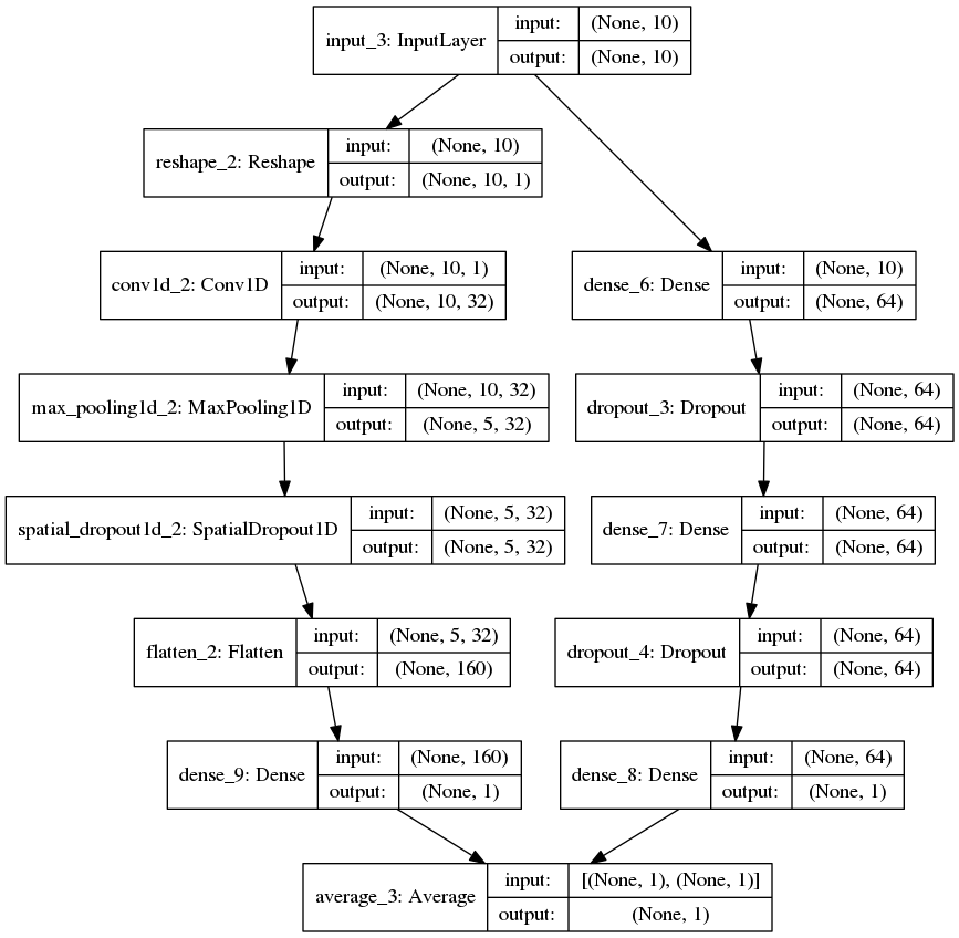
In the post (https://statcompute.wordpress.com/2017/01/08/an-example-of-merge-layer-in-keras), it was shown how to build a merge-layer DNN by using the Keras Sequential model. In the example below, I tried to scratch a merge-layer DNN with the Keras functional API in both R and Python. In particular, the merge-layer DNN is the average of a multilayer perceptron network and a 1D convolutional network, just for fun and curiosity. Since the purpose of this exercise is to explore the network structure and the use case of Keras API, I didn’t bother to mess around with parameters.


library(keras)
df <- read.csv("credit_count.txt")
Y <- matrix(df[df$CARDHLDR == 1, ]$DEFAULT)
X <- scale(df[df$CARDHLDR == 1, ][3:14])
inputs <- layer_input(shape = c(ncol(X)))
mlp <- inputs %>%
layer_dense(units = 64, activation = 'relu', kernel_initializer = 'he_uniform') %>%
layer_dropout(rate = 0.2, seed = 1) %>%
layer_dense(units = 64, activation = 'relu', kernel_initializer = 'he_uniform') %>%
layer_dropout(rate = 0.2, seed = 1) %>%
layer_dense(1, activation = 'sigmoid')
cnv <- inputs %>%
layer_reshape(c(ncol(X), 1)) %>%
layer_conv_1d(32, 4, activation = 'relu', padding = "same", kernel_initializer = 'he_uniform') %>%
layer_max_pooling_1d(2) %>%
layer_spatial_dropout_1d(0.2) %>%
layer_flatten() %>%
layer_dense(1, activation = 'sigmoid')
avg <- layer_average(c(mlp, cnv))
mdl <- keras_model(inputs = inputs, outputs = avg)
mdl %>% compile(optimizer = optimizer_sgd(lr = 0.1, momentum = 0.9), loss = 'binary_crossentropy', metrics = c('binary_accuracy'))
mdl %>% fit(x = X, y = Y, epochs = 50, batch_size = 1000, verbose = 0)
mdl %>% predict(x = X)

view raw

keras_average.R

hosted with ❤ by GitHub


from numpy.random import seed
from pandas import read_csv, DataFrame
from sklearn.preprocessing import scale
from keras.layers.convolutional import Conv1D, MaxPooling1D
from keras.layers.merge import average
from keras.layers import Input, Dense, Flatten, Reshape, Dropout, SpatialDropout1D
from keras.models import Model
from keras.optimizers import SGD
from keras.utils import plot_model
df = read_csv("credit_count.txt")
Y = df[df.CARDHLDR == 1].DEFAULT
X = scale(df[df.CARDHLDR == 1].iloc[:, 2:12])
D = 0.2
S = 1
seed(S)
### INPUT DATA
inputs = Input(shape = (X.shape[1],))
### DEFINE A MULTILAYER PERCEPTRON NETWORK
mlp_net = Dense(64, activation = 'relu', kernel_initializer = 'he_uniform')(inputs)
mlp_net = Dropout(rate = D, seed = S)(mlp_net)
mlp_net = Dense(64, activation = 'relu', kernel_initializer = 'he_uniform')(mlp_net)
mlp_net = Dropout(rate = D, seed = S)(mlp_net)
mlp_out = Dense(1, activation = 'sigmoid')(mlp_net)
mlp_mdl = Model(inputs = inputs, outputs = mlp_out)
### DEFINE A CONVOLUTIONAL NETWORK
cnv_net = Reshape((X.shape[1], 1))(inputs)
cnv_net = Conv1D(32, 4, activation = 'relu', padding = "same", kernel_initializer = 'he_uniform')(cnv_net)
cnv_net = MaxPooling1D(2)(cnv_net)
cnv_net = SpatialDropout1D(D)(cnv_net)
cnv_net = Flatten()(cnv_net)
cnv_out = Dense(1, activation = 'sigmoid')(cnv_net)
cnv_mdl = Model(inputs = inputs, outputs = cnv_out)
### COMBINE MLP AND CNV
con_out = average([mlp_out, cnv_out])
con_mdl = Model(inputs = inputs, outputs = con_out)
sgd = SGD(lr = 0.1, momentum = 0.9)
con_mdl.compile(optimizer = sgd, loss = 'binary_crossentropy', metrics = ['binary_accuracy'])
con_mdl.fit(X, Y, batch_size = 2000, epochs = 50, verbose = 0)
plot_model(con_mdl, to_file = 'model.png', show_shapes = True, show_layer_names = True)

model

XFrames: Another Convenient Python Interface to Spark

Currently, pyspark might be the most popular python interface to Apache Spark. However, the xframes package (https://github.com/cchayden/xframes) definitely is an alternative worth trying.

As shown in the code snippet below, the XFrame, which is the dataframe object in the xframes package, interacts well with other python data structures and numpy functions. To me, the XFrame is easier to work with than the pyspark.dataframe and has more “authentic” python flavor.

from xframes import XFrame, aggregate

df = XFrame.read_csv("Downloads/nycflights.csv", header = True, nrows = 11)

### SUBSETTING
sel_cols = ["origin", "dest", "distance", "dep_delay", "carrier"]

df2 = df[sel_cols]
# OR:
# df.sql("select " + ", ".join(sel_cols) + " from df")

### FILTERING ###
print df2[(df2["origin"] == 'EWR') & (df2["carrier"] == "UA")]
# OR:
# print df2.filterby("EWR", "origin").filterby("UA", "carrier")

### AGGREGATING ###
from numpy import median

grp1 = df2.groupby("origin", {"dist": aggregate.CONCAT("distance")})

agg1 = XFrame({"origin": grp1["origin"], "med_dist": map(median, grp1["dist"])})
# OR:
# grp1["med_dist"] = grp1.apply(lambda row: median(row["dist"]))
# agg1 = grp1[["origin", "med_dist"]]
# USING SQL:
# df2.sql("select origin, percentile_approx(distance, 0.5) as med_dist from df2 group by origin")

for row in agg1:
  print row
# {'origin': u'LGA', 'med_dist': 747.5}
# {'origin': u'JFK', 'med_dist': 1089.0}
# {'origin': u'EWR', 'med_dist': 1065.0}

agg2 = df2.groupby("origin", {"avg_delay": aggregate.MEAN("dep_delay")})
# USING SQL:
# df2.sql("select origin, mean(dep_delay) as avg_delay from df2 group by origin")

for row in agg2:
  print row
# {'origin': u'LGA', 'avg_delay': -1.75}
# {'origin': u'JFK', 'avg_delay': -0.6666666666666666}
# {'origin': u'EWR', 'avg_delay': -2.3333333333333335}

### JOINING ###
for row in  agg1.join(agg2, on = {"origin": "origin"}, how = "inner"):
    print row
# {'origin': u'LGA', 'med_dist': 747.5, 'avg_delay': -1.75}
# {'origin': u'JFK', 'med_dist': 1089.0, 'avg_delay': -0.6666666666666666}
# {'origin': u'EWR', 'med_dist': 1065.0, 'avg_delay': -2.3333333333333335}

Data Wrangling with Astropy Package

from astropy.io import ascii

from astropy.table import Table, join

from numpy import nanmean, nanmedian, array, sort

tbl1 = ascii.read("Downloads/nycflights.csv", format = "csv")

### SUBSETTING
sel_cols = ["origin", "dest", "distance", "dep_delay", "carrier"]

tbl2 = tbl1[sel_cols][range(10)]

tbl2.info
#   name   dtype
#--------- -----
#   origin  str3
#     dest  str3
# distance int64
#dep_delay int64
#  carrier  str2

### FILTERING ###
tbl2[list(i["carrier"] == "UA" and i["origin"] == 'EWR' for i in tbl2)]
#origin dest distance dep_delay carrier
#------ ---- -------- --------- -------
#   EWR  IAH     1400         2      UA
#   EWR  ORD      719        -4      UA

tbl2[(tbl2["carrier"] == "UA") & (tbl2["origin"] == "EWR")]
#origin dest distance dep_delay carrier
#------ ---- -------- --------- -------
#   EWR  IAH     1400         2      UA
#   EWR  ORD      719        -4      UA

### FILTER BY GROUPS ###
vstack(map(lambda x: x[(x["carrier"] == "UA") & (x["origin"] == "EWR")],
           tbl2.group_by(sort(array(range(len(tbl2))) % 2)).groups))
#origin dest distance dep_delay carrier
#------ ---- -------- --------- -------
#   EWR  IAH     1400         2      UA
#   EWR  ORD      719        -4      UA

### GROUPING ###
grp = tbl2.group_by("origin")

### AGGREGATING ###
agg1 = Table(grp['origin', 'distance'].groups.aggregate(nanmedian), names = ["origin", "med_dist"])
#origin med_dist
#------ --------
#   EWR   1065.0
#   JFK   1089.0
#   LGA    747.5

agg2 = Table(grp['origin', 'dep_delay'].groups.aggregate(nanmean), names = ["origin", "avg_delay"])
#origin      avg_delay
#------ -------------------
#   EWR -2.3333333333333335
#   JFK -0.6666666666666666
#   LGA               -1.75

### JOINING ###
join(agg1, agg2, join_type = "inner", keys = "origin")
#origin med_dist      avg_delay
#------ -------- -------------------
#   EWR   1065.0 -2.3333333333333335
#   JFK   1089.0 -0.6666666666666666
#   LGA    747.5               -1.75

Manipulating Dictionary List with SQLite Back-End


from astropy.io.ascii import read

selected = ["origin", "dep_delay", "distance"]

csv = read("Downloads/nycflights.csv", format = 'csv', data_end = 11)[selected]

lst = map(lambda x: dict(zip(x.colnames, x)), csv)

from dataset import connect

### CREATE IN-MEMORY SQLITE DB ###
db = connect('sqlite:///:memory:', row_type = dict)

tbl = db.create_table("tbl", primary_id = False)

tbl.insert_many(lst)

list(db.query("select * from tbl limit 3"))
# [{u'dep_delay': 2, u'distance': 1400, u'origin': u'EWR'},
#  {u'dep_delay': 4, u'distance': 1416, u'origin': u'LGA'},
#  {u'dep_delay': 2, u'distance': 1089, u'origin': u'JFK'}]

sum1 = db.create_table("sum1", primary_id = False)

from numpy import nanmedian

sum1.insert_many(
  map(lambda x: dict(origin = x,
                     med_dist = nanmedian([i["distance"] for i in
                       db.query("select distance from tbl where origin = :origin", {"origin": x})])),
      [i["origin"] for i in db.query("select distinct origin from tbl")]))

sum2 = db.create_table("sum2", primary_id = False)

sum2.insert_many(list(db.query("select origin, ROUND(AVG(dep_delay), 2) as avg_delay from tbl group by origin")))

list(db.query("select a.*, b.avg_delay from sum1 as a, sum2 as b where a.origin = b.origin"))
#[{u'avg_delay': -2.33, u'med_dist': 1065.0, u'origin': u'EWR'},
# {u'avg_delay': -1.75, u'med_dist': 747.5, u'origin': u'LGA'},
# {u'avg_delay': -0.67, u'med_dist': 1089.0, u'origin': u'JFK'}]

Joining Dictionary Lists by Key

### IMPORT AND PREPARE THE DATA ###
from astropy.io.ascii import read

selected = ["origin", "dep_delay", "distance"]

tbl = read("Downloads/nycflights.csv", format = 'csv', data_end = 11)[selected]

lst = map(lambda x: dict(zip(x.colnames, x)), tbl)

key = set(map(lambda x: x["origin"], lst))

grp = dict(map(lambda x: (x, [i for i in lst if i["origin"] == x]), key))

#   ALTERNATIVELY, USE CLJ.SEQS.GROUP_BY()
# from clj.seqs import group_by
# group_by(lambda x: x["origin"], lst)
#   OR TOOLZ.ITERTOOLZ.GROUPBY()
# from toolz import itertoolz
# itertoolz.groupby("origin", lst)
#   OR ITERTOOLS.GROUPBY()
# key_fn = lambda x: x["origin"]
# dict((k, list(g)) for k, g in groupby(sorted(lst, key = key_fn), key_fn))

### CREATE 2 DICTIONARY LISTS TO BE MERGED ###
from numpy import nanmean, nanmedian

l1 = list({"origin"   : k,
           "med_dist" : nanmedian([v["distance"] for v in grp[k]])
          } for k in grp.keys())
#[{'med_dist': 1089.0, 'origin': 'JFK'},
# {'med_dist': 1065.0, 'origin': 'EWR'},
# {'med_dist': 747.5, 'origin': 'LGA'}]

l2 = list({"origin"   : k,
           "avg_delay": round(nanmean(map(lambda v: v["dep_delay"], grp[k])), 2)
          } for k in grp.keys())
#[{'avg_delay': -0.67, 'origin': 'JFK'},
# {'avg_delay': -2.33, 'origin': 'EWR'},
# {'avg_delay': -1.75, 'origin': 'LGA'}]

### METHOD 1: LIST COMPREHENSION ###
join1 = list(dict(v1, **v2) for v2 in l2 for v1 in l1 if v1["origin"] == v2["origin"])

### METHOD 2: CARTESIAN PRODUCT WITH ITERTOOLS.PRODUCT() ###
from itertools import product

join2 = list(dict(d1, **d2) for d1, d2 in product(l1, l2) if d1["origin"] == d2["origin"])

### METHOD 3: AD-HOC FUNCTION WITH DICT COPY() AND UPDATE() METHODS ###
def join_fn(x, y, key):
  result = list()
  for i, j in group_by(lambda x: x[key], x + y).values():
    xy = i.copy()
    xy.update(j)
    result.append(xy)
  return result

join3 = join_fn(l1, l2, "origin")

### METHOD 4: DEFAULTDICT() ###
from collections import defaultdict

dd = defaultdict(dict)

for x in l1 + l2:
  dd[x["origin"]].update(x)

join4 = dd.values()

### METHOD 5: ORDEREDDICT() ###
from collections import OrderedDict

od = OrderedDict()

for x in l1 + l2:
  if x["origin"] in od:
    od[x["origin"]].update(x)
  else:
    od[x["origin"]] = x

join5 = od.values()

### METHOD 6:  ###
from toolz import itertoolz, dicttoolz

join6 = list(dicttoolz.merge(i, j) for i, j in  itertoolz.join("origin", l1, "origin", l2))

# EXPECTED OUTPUT:
# [{'avg_delay': -0.67, 'med_dist': 1089.0, 'origin': 'JFK'},
#  {'avg_delay': -2.33, 'med_dist': 1065.0, 'origin': 'EWR'},
#  {'avg_delay': -1.75, 'med_dist': 747.5, 'origin': 'LGA'}]

Aggregation of Dictionary List by Key

from astropy.io.ascii import read

from numpy import nanmean, nanmedian, vectorize

selected = ["origin", "dep_delay", "distance"]

tbl = read("Downloads/nycflights.csv", format = 'csv', data_end = 11)[selected]

lst = map(lambda x: dict(zip(x.colnames, x)), tbl)

key = set([x["origin"] for x in lst])

grp = map(lambda x: {x: list(i for i in lst if i["origin"] == x)}, key)

### USING LIST COMPREHENSION ###
list({"origin"    : x.keys()[0],
      "flight_nbr": len(x.values()[0]),
      "med_dist"  : nanmedian([i["distance"] for i in x.values()[0]]),
      "avg_delay" : round(nanmean([i["dep_delay"] for i in x.values()[0]]), 2)
      } for x in grp)

### USING MAP() ALTERNATIVELY ###
map(lambda x: {"origin"    : x.keys()[0],
               "flight_nbr": len(x.values()[0]),
               "med_dist"  : nanmedian([i["distance"] for i in x.values()[0]]),
               "avg_delay" : round(nanmean([i["dep_delay"] for i in x.values()[0]]), 2)}, grp)

### USING VECTORIZE() ###
def agg(x):
  return({"origin"    : x.keys()[0],
          "flight_nbr": len(x.values()[0]),
          "med_dist"  : nanmedian([i["distance"] for i in x.values()[0]]),
          "avg_delay" : round(nanmean([i["dep_delay"] for i in x.values()[0]]), 2)})

list(vectorize(agg)(grp))

# RESULT:
# [{'avg_delay': -0.67, 'flight_nbr': 3, 'med_dist': 1089.0, 'origin': 'JFK'},
#  {'avg_delay': -2.33, 'flight_nbr': 3, 'med_dist': 1065.0, 'origin': 'EWR'},
#  {'avg_delay': -1.75, 'flight_nbr': 4, 'med_dist': 747.5, 'origin': 'LGA'}]

Convert SAS Dataset to Dictionary List

from sas7bdat import SAS7BDAT

with SAS7BDAT("Downloads/accepts.sas7bdat") as f:
  lst = map(lambda x: dict(zip(f.column_names, x)), [i for i in f][1:])

col = ["app_id", "bureau_score", "ltv", "tot_derog", "tot_income", "bad"]

for i in range(5):
  print {k: lst[i].get(k) for k in col}

#{'tot_income': 4800.0, 'ltv': 109.0, 'app_id': 1001.0, 'bureau_score': 747.0, 'bad': 0.0, 'tot_derog': 6.0}
#{'tot_income': 5833.33, 'ltv': 97.0, 'app_id': 1002.0, 'bureau_score': 744.0, 'bad': 0.0, 'tot_derog': 0.0}
#{'tot_income': 2308.33, 'ltv': 105.0, 'app_id': 1003.0, 'bureau_score': 667.0, 'bad': 0.0, 'tot_derog': 0.0}
#{'tot_income': 4083.33, 'ltv': 78.0, 'app_id': 1005.0, 'bureau_score': 648.0, 'bad': 1.0, 'tot_derog': 2.0}
#{'tot_income': 5783.33, 'ltv': 100.0, 'app_id': 1006.0, 'bureau_score': 649.0, 'bad': 0.0, 'tot_derog': 2.0}

Grouping Dictionary List by Key

It is shown in code snippets below how to group a dictionary list based on a specific key.

First of all, let’s import the data from a csv file.

from astropy.io.ascii import read

selected = ["origin", "dest", "distance", "carrier"]

### IMPORT CSV FILE INTO ASTROPY TABLE ###
tbl = read("Downloads/nycflights.csv", format = 'csv', data_end = 11)[selected]

### CONVERT ASTROPY TABLE TO DICTIONARY LIST ###
lst = map(lambda x: dict(zip(x.colnames, x)), tbl)

### DISPLAY DATA CONTENTS ###
from tabulate import tabulate

print tabulate([lst[i] for i in range(3)], headers = "keys", tablefmt = "fancy_grid")

╒══════════╤════════╤═══════════╤════════════╕
│ origin   │ dest   │ carrier   │   distance │
╞══════════╪════════╪═══════════╪════════════╡
│ EWR      │ IAH    │ UA        │       1400 │
├──────────┼────────┼───────────┼────────────┤
│ EWR      │ ORD    │ UA        │        719 │
├──────────┼────────┼───────────┼────────────┤
│ EWR      │ FLL    │ B6        │       1065 │
╘══════════╧════════╧═══════════╧════════════╛

In the first approach, only standard Python modules and data structures are used.

### APPROACH 1: HOMEBREW GROUPING ###

from operator import itemgetter

### GET UNIQUE VALUES OF GROUP KEY ###
g_key = set([x["origin"] for x in lst])

### GROUPING LIST BY GROUP KEY ###
g_lst1 = sorted(map(lambda x: (x, [i for i in lst if i["origin"] == x]), g_key), key = itemgetter(0))

for i in g_lst1:
  print tabulate(i[1], headers = "keys", tablefmt = "fancy_grid")

In the second approach, we first sort the list by the key and then group the list with the itertools.groupby() function.

### APPROACH 2: ITERTOOLS.GROUPBY  ###

### SORTING DICTIONARY BEFORE GROUPING ###
s_lst = sorted(lst, key = itemgetter('origin'))

### GROUPING DICTIONARY BY "ORIGIN" ###
from itertools import groupby

g_lst2 = [(k, list(g)) for k, g in groupby(s_lst, itemgetter("origin"))]

for i in g_lst2:
  print tabulate(i[1], headers = "keys", tablefmt = "fancy_grid")

In the third approach, we use the defaultdict class in the collections module.

### APPROACH 3: DEFAULTDICT ###

from collections import defaultdict

### CREATE KEY-VALUE PAIRS FROM LIST ###
ddata = [(x["origin"], x) for x in lst]

### CREATE DEFAULTDICT ###
ddict = defaultdict(list)

for key, value in ddata:
  ddict[key].append(value)

g_lst3 = sorted(ddict.items(), key = itemgetter(0))

for i in g_lst3:
  print tabulate(i[1], headers = "keys", tablefmt = "fancy_grid")

In the fourth approach, we use the ordereddict class also in the collections module.

### APPROACH 4: ORDEREDDICT ###
from collections import OrderedDict

odict = OrderedDict()

for key, value in ddata:
  if key in odict: odict[key].append(value)
  else: odict[key] = [value]

g_lst4 = sorted(odict.items(), key = itemgetter(0))

for i in g_lst4:
  print tabulate(i[1], headers = "keys", tablefmt = "fancy_grid")

In the output below, it is shown that four grouped lists are identical.


g_lst1 == g_lst2 == g_lst3 == g_lst4
# True

╒══════════╤════════╤═══════════╤════════════╕
│ origin   │ dest   │ carrier   │   distance │
╞══════════╪════════╪═══════════╪════════════╡
│ EWR      │ IAH    │ UA        │       1400 │
├──────────┼────────┼───────────┼────────────┤
│ EWR      │ ORD    │ UA        │        719 │
├──────────┼────────┼───────────┼────────────┤
│ EWR      │ FLL    │ B6        │       1065 │
╘══════════╧════════╧═══════════╧════════════╛
╒══════════╤════════╤═══════════╤════════════╕
│ origin   │ dest   │ carrier   │   distance │
╞══════════╪════════╪═══════════╪════════════╡
│ JFK      │ MIA    │ AA        │       1089 │
├──────────┼────────┼───────────┼────────────┤
│ JFK      │ BQN    │ B6        │       1576 │
├──────────┼────────┼───────────┼────────────┤
│ JFK      │ MCO    │ B6        │        944 │
╘══════════╧════════╧═══════════╧════════════╛
╒══════════╤════════╤═══════════╤════════════╕
│ origin   │ dest   │ carrier   │   distance │
╞══════════╪════════╪═══════════╪════════════╡
│ LGA      │ IAH    │ UA        │       1416 │
├──────────┼────────┼───────────┼────────────┤
│ LGA      │ ATL    │ DL        │        762 │
├──────────┼────────┼───────────┼────────────┤
│ LGA      │ IAD    │ EV        │        229 │
├──────────┼────────┼───────────┼────────────┤
│ LGA      │ ORD    │ AA        │        733 │
╘══════════╧════════╧═══════════╧════════════╛

Subset Dictionary by Values

from csv import DictReader

selected = ["origin", "dest", "distance", "carrier"]

with open("Downloads/nycflights.csv") as f:
  d = DictReader(f)
  l = map(lambda d: {k: d[k] for k in selected}, [next(d) for i in xrange(10)])

from pandas import DataFrame

from sys import getsizeof

### COMPARING OBJECT SIZES BETWEEN A DATAFRAME AND A LIST ###
float(getsizeof(DataFrame(l))) / getsizeof(l)
# 13.282894736842104

from tabulate import tabulate

print tabulate([l[i] for i in range(3)], headers = "keys")
# origin    dest    carrier      distance
# --------  ------  ---------  ----------
# EWR       IAH     UA               1400
# LGA       IAH     UA               1416
# JFK       MIA     AA               1089

### SOLUTION 1: LIST COMPREHENSION ###
list(x for x in l if x["origin"] == 'JFK' and x["carrier"] == 'B6')

### SOLUTION 2: FILTER() FUNCTION ###
filter(lambda x: x["origin"] == 'JFK' and x["carrier"] == 'B6', l)

### SOLUTION 3: MAP() AND LAMBDA() FUNCTIONS ###
list(v for v, i in map(lambda x: (x, x['origin'] == 'JFK' and x["carrier"] == 'B6'), l) if i)

### SOLUTION 4: CREATE A CLASS ###
class subset:
  def __init__(self, lst, expr):
    self.result = []
    for x in lst:
      if eval(expr):
        self.result.append(x)

subset(l, 'x["origin"] == "JFK" and x["carrier"] == "B6"').result

### SOLUTION 5: LIST_DICT_DB MODULE ###
from list_dict_DB import list_dict_DB as dict2db
db = dict2db(l)
db.query(origin = 'JFK', carrier = 'B6')

# EXPECTED OUTCOME:
# [{'carrier': 'B6', 'dest': 'BQN', 'distance': '1576', 'origin': 'JFK'},
#  {'carrier': 'B6', 'dest': 'MCO', 'distance': '944', 'origin': 'JFK'}]

Subset Dictionary by Keys

### READ A DATA SAMPLE WITH THREE RECORDS FROM THE CSV FILE
from csv import DictReader

with open("Downloads/nycflights.csv") as f:
  d = DictReader(f)
  l = [next(d) for i in xrange(3)]

### GET A DICT FROM THE LIST
d = l[0]

### SHOW KEYS OF THE DICT
print d.keys()
#['origin', 'dep_time', 'flight', 'hour', 'dep_delay', 'distance', 'dest', 'month', 'air_time', 'carrier', 'year', 'arr_delay', 'tailnum', 'arr_time', 'day', 'minute']

### SELECTED KEYS
selected = ["origin", "dest", "distance", "carrier"]

# EXPECTED OUTPUT 
# {'carrier': 'UA', 'dest': 'IAH', 'distance': '1400', 'origin': 'EWR'}

### METHOD 1: DEFINE BY THE DICT COMPREHENSION

{k: d[k] for k in selected}

{k: d.get(k) for k in selected}

{k: v for k, v in d.items() if k in selected}

### METHOD 2: DEFINE BY THE DICT CONSTRUCTOR

dict((k, d[k]) for k in selected)

dict(map(lambda k: (k, d[k]), selected))

dict(filter(lambda i: i[0] in selected, d.items()))

### METHOD 3: DEFINE WITH THE ZIP() FUNCTION

dict(zip(selected, [d[k] for k in selected]))

# ITEMGETTER() FUNCTION WITH THE UNPACK OPERATOR (*)
from operator import itemgetter
dict(zip(selected, itemgetter(*selected)(d)))

# AT() FUNCTION WITH THE UNPACK OPERATOR (*)
from pydash import at
dict(zip(selected, at(d, *selected)))

### APPLY ABOVE LOGIC TO THE WHOLE LIST OF DICTIONARIES
### WITH THE MAP FUNCTION
map(lambda d: {k: d[k] for k in selected}, l)

### ALTERNATIVELY, WITH THE LIST COMPREHENSION
[(lambda x: {k: x[k] for k in selected})(d) for d in l]

### OR THE PARALLEL POOL.MAP() FUNCTION
# ALWAYS DEFINE THE FUNCTION FIRST
def sel(d):
  return({k: d[k] for k in selected})

# THE MULTIPROCESSING MODULE NEXT
from multiprocessing import Pool, cpu_count
from contextlib import closing

with closing(Pool(processes = cpu_count())) as pool:
  pool.map(sel, l)
  pool.terminate()

# OUTPUT:
# [{'carrier': 'UA', 'dest': 'IAH', 'distance': '1400', 'origin': 'EWR'},
#  {'carrier': 'UA', 'dest': 'IAH', 'distance': '1416', 'origin': 'LGA'},
#  {'carrier': 'AA', 'dest': 'MIA', 'distance': '1089', 'origin': 'JFK'}]

Import CSV as Dictionary List

When the DictReader() function in the csv module is used to read the csv file as a list of dictionaries in python, numbers would be imported as strings, as shown below.


from csv import DictReader

from pprint import pprint

### EXAMINE 3 ROWS OF DATA
with open("Downloads/nycflights.csv") as f:
  d = DictReader(f)
  l = [next(d) for i in xrange(3)]

pprint(l[0])
#{'air_time': '227',
# 'arr_delay': '11',
# 'arr_time': '830',
# 'carrier': 'UA',
# 'day': '1',
# 'dep_delay': '2',
# 'dep_time': '517',
# 'dest': 'IAH',
# 'distance': '1400',
# 'flight': '1545',
# 'hour': '5',
# 'minute': '17',
# 'month': '1',
# 'origin': 'EWR',
# 'tailnum': 'N14228',
# 'year': '2013'}

A solution to address the aforementioned issue is first to import the csv file into a Pandas DataFrame and then to convert the DataFrame to the list of dictionaries, as shown in the code snippet below.


from pandas import read_csv

from numpy import array_split

from multiprocessing import Pool, cpu_count

n = 1000

d = read_csv("Downloads/nycflights.csv", nrows = n)

%time l1 = [dict(zip(d.iloc[i].index.values, d.iloc[i].values)) for i in range(len(d))]
#CPU times: user 396 ms, sys: 39.9 ms, total: 436 ms
#Wall time: 387 ms

pprint(l1[0])
#{'air_time': 227.0,
# 'arr_delay': 11.0,
# 'arr_time': 830.0,
# 'carrier': 'UA',
# 'day': 1,
# 'dep_delay': 2.0,
# 'dep_time': 517.0,
# 'dest': 'IAH',
# 'distance': 1400,
# 'flight': 1545,
# 'hour': 5.0,
# 'minute': 17.0,
# 'month': 1,
# 'origin': 'EWR',
# 'tailnum': 'N14228',
# 'year': 2013}

In addition to using the list comprehension as shown above, we can also split the DataFrame into pieces and then apply the MapReduce paradigm together with lambda functions.


d2 = array_split(d, 4, axis = 0)

%%time
l2 = reduce(lambda a, b: a + b,
       map(lambda df: [dict(zip(df.iloc[i].index.values, df.iloc[i].values)) for i in range(len(df))], d2))
#CPU times: user 513 ms, sys: 83.3 ms, total: 596 ms
#Wall time: 487 ms

Alternatively, we could also apply the parallelism with the multiprocessing module. As shown in the benchmark, the parallel version is much more efficient than the sequential version.


def p2dict(df):
  return([dict(zip(df.iloc[i].index.values, df.iloc[i].values)) for i in range(len(df))])

pool = Pool(processes = cpu_count())

%time l3 = reduce(lambda a, b: a + b, pool.map(p2dict, d2))
#CPU times: user 12.5 ms, sys: 23 µs, total: 12.5 ms
#Wall time: 204 ms

pool.close()

In addition to using Pandas, we can also consider the astropy module. As shown in the code snippet, albeit slightly slower than Pandas, astropy is much cleaner and more intuitive.


from astropy.io.ascii import read

a = read("Downloads/nycflights.csv", format = 'csv', data_end = n + 1)

def a2dict(row):
  return(dict(zip(row.colnames, row)))

pool = Pool(processes = cpu_count())

%time l4 = pool.map(a2dict, a)
#CPU times: user 90.6 ms, sys: 4.47 ms, total: 95.1 ms
#Wall time: 590 ms

pool.close()

Sparkling Water and Moving Data Around

Sparkling Water is an application to integrate H2O with Spark. Below is an example showing how to move the data around among Pandas DataFrame, H2OFrame, and Spark Dataframe.

1. Define Context

In [1]: from pandas import read_csv, DataFrame

In [2]: from pyspark import sql

In [3]: from pysparkling import H2OContext

In [4]: from h2o import import_file, H2OFrame

In [5]: ss = sql.SparkSession.builder.getOrCreate()

In [6]: hc = H2OContext.getOrCreate(ss)

2. Convert Pandas Dataframe to H2OFrame and Spark DataFrame

In [7]: p_df = read_csv("Documents/credit_count.txt")

In [8]: type(p_df)
Out[8]: pandas.core.frame.DataFrame

In [9]: p2s_df = ss.createDataFrame(p_df)

In [10]: type(p2s_df)
Out[10]: pyspark.sql.dataframe.DataFrame

In [11]: p2h_df = H2OFrame(p_df)

In [12]: type(p2h_df)
Out[12]: h2o.frame.H2OFrame

3. Convert Spark Dataframe to H2OFrame and Pandas DataFrame

In [13]: s_df = ss.read.csv("Documents/credit_count.txt", header = True, inferSchema = True)

In [14]: type(s_df)
Out[14]: pyspark.sql.dataframe.DataFrame

In [15]: s2p_df = s_df.toPandas()

In [16]: type(s2p_df)
Out[16]: pandas.core.frame.DataFrame

In [17]: s2h_df = hc.as_h2o_frame(s_df)

In [18]: type(s2h_df)
Out[18]: h2o.frame.H2OFrame

4. Convert H2OFrame to Pandas Dataframe and Spark DataFrame

In [19]: h_df = import_file("Documents/credit_count.txt", header = 1, sep = ",")

In [20]: type(h_df)
Out[20]: h2o.frame.H2OFrame

In [21]: h2p_df = h_df.as_data_frame()

In [22]: type(h2p_df)
Out[22]: pandas.core.frame.DataFrame

In [23]: h2s_df = hc.as_spark_frame(h_df)

In [24]: type(h2s_df)
Out[24]: pyspark.sql.dataframe.DataFrame

A Simple Convolutional Neural Network for The Binary Outcome

Since CNN(Convolutional Neural Networks) have achieved a tremendous success in various challenging applications, e.g. image or digit recognitions, one might wonder how to employ CNNs in classification problems with binary outcomes.

Below is an example showing how to use a simple 1D convolutional neural network to predict credit card defaults.

### LOAD PACKAGES 
from numpy.random import seed
from pandas import read_csv, DataFrame
from sklearn.preprocessing import minmax_scale
from keras.layers.convolutional import Conv1D, MaxPooling1D
from keras.optimizers import SGD
from keras.models import Sequential
from keras.layers import Dense, Flatten

### PREPARE THE DATA 
df = read_csv("credit_count.txt")
Y = df[df.CARDHLDR == 1].DEFAULT
X = minmax_scale(df[df.CARDHLDR == 1].ix[:, 2:12], axis = 0)
y_train = Y.values
x_train = X.reshape(X.shape[0], X.shape[1], 1)

### FIT A 1D CONVOLUTIONAL NEURAL NETWORK
seed(2017)
conv = Sequential()
conv.add(Conv1D(20, 4, input_shape = x_train.shape[1:3], activation = 'relu'))
conv.add(MaxPooling1D(2))
conv.add(Flatten())
conv.add(Dense(1, activation = 'sigmoid'))
sgd = SGD(lr = 0.1, momentum = 0.9, decay = 0, nesterov = False)
conv.compile(loss = 'binary_crossentropy', optimizer = sgd, metrics = ['accuracy'])
conv.fit(x_train, y_train, batch_size = 500, epochs = 100, verbose = 0)

Considering that 1D is the special case of 2D, we can also solve the same problem with a 2D convolutional neural network by changing the input shape, as shown below.

from numpy.random import seed
from pandas import read_csv, DataFrame
from sklearn.preprocessing import minmax_scale
from keras_diagram import ascii
from keras.layers.convolutional import Conv2D, MaxPooling2D
from keras.optimizers import SGD
from keras.models import Sequential
from keras.layers import Dense, Flatten

df = read_csv("credit_count.txt")
Y = df[df.CARDHLDR == 1].DEFAULT
X = minmax_scale(df[df.CARDHLDR == 1].ix[:, 2:12], axis = 0)
y_train = Y.values
x_train = X.reshape(X.shape[0], 1, X.shape[1], 1)

seed(2017)
conv = Sequential()
conv.add(Conv2D(20, (1, 4), input_shape = x_train.shape[1:4], activation = 'relu'))
conv.add(MaxPooling2D((1, 2)))
conv.add(Flatten())
conv.add(Dense(1, activation = 'sigmoid'))
sgd = SGD(lr = 0.1, momentum = 0.9, decay = 0, nesterov = False)
conv.compile(loss = 'binary_crossentropy', optimizer = sgd, metrics = ['accuracy'])
conv.fit(x_train, y_train, batch_size = 500, epochs = 100, verbose = 0)

Autoencoder for Dimensionality Reduction

We often use ICA or PCA to extract features from the high-dimensional data. The autoencoder is another interesting algorithm to achieve the same purpose in the context of Deep Learning.

With the purpose of learning a function to approximate the input data itself such that F(X) = X, an autoencoder consists of two parts, namely encoder and decoder. While the encoder aims to compress the original input data into a low-dimensional representation, the decoder tries to reconstruct the original input data based on the low-dimension representation generated by the encoder. As a result, the autoencoder has been widely used to remove the data noise as well to reduce the data dimension.

First of all, we will show the basic structure of an autoencoder with 1-layer encoder and 1-layer decoder, as below. In the example, we will compress the input data with 10 columns into a compressed on with 3 columns.

from pandas import read_csv, DataFrame
from numpy.random import seed
from sklearn.preprocessing import minmax_scale
from sklearn.model_selection import train_test_split
from keras.layers import Input, Dense
from keras.models import Model

df = read_csv("credit_count.txt")
Y = df[df.CARDHLDR == 1].DEFAULTS
X = df[df.CARDHLDR == 1].ix[:, 2:12]
# SCALE EACH FEATURE INTO [0, 1] RANGE
sX = minmax_scale(X, axis = 0)
ncol = sX.shape[1]
X_train, X_test, Y_train, Y_test = train_test_split(sX, Y, train_size = 0.5, random_state = seed(2017))

### AN EXAMPLE OF SIMPLE AUTOENCODER ###
# InputLayer (None, 10)
#      Dense (None, 5)
#      Dense (None, 10)

input_dim = Input(shape = (ncol, ))
# DEFINE THE DIMENSION OF ENCODER ASSUMED 3
encoding_dim = 3
# DEFINE THE ENCODER LAYER
encoded = Dense(encoding_dim, activation = 'relu')(input_dim)
# DEFINE THE DECODER LAYER
decoded = Dense(ncol, activation = 'sigmoid')(encoded)
# COMBINE ENCODER AND DECODER INTO AN AUTOENCODER MODEL
autoencoder = Model(input = input_dim, output = decoded)
# CONFIGURE AND TRAIN THE AUTOENCODER
autoencoder.compile(optimizer = 'adadelta', loss = 'binary_crossentropy')
autoencoder.fit(X_train, X_train, nb_epoch = 50, batch_size = 100, shuffle = True, validation_data = (X_test, X_test))
# THE ENCODER TO EXTRACT THE REDUCED DIMENSION FROM THE ABOVE AUTOENCODER
encoder = Model(input = input_dim, output = encoded)
encoded_input = Input(shape = (encoding_dim, ))
encoded_out = encoder.predict(X_test)
encoded_out[0:2]
#array([[ 0.        ,  1.26510417,  1.62803197],
#       [ 2.32508397,  0.99735016,  2.06461048]], dtype=float32)

In the next example, we will relax the constraint of layers and employ a stack of layers to achievement the same purpose as above.

### AN EXAMPLE OF DEEP AUTOENCODER WITH MULTIPLE LAYERS
# InputLayer (None, 10)
#      Dense (None, 20)
#      Dense (None, 10)
#      Dense (None, 5)
#      Dense (None, 3)
#      Dense (None, 5)
#      Dense (None, 10)
#      Dense (None, 20)
#      Dense (None, 10)

input_dim = Input(shape = (ncol, ))
# DEFINE THE DIMENSION OF ENCODER ASSUMED 3
encoding_dim = 3
# DEFINE THE ENCODER LAYERS
encoded1 = Dense(20, activation = 'relu')(input_dim)
encoded2 = Dense(10, activation = 'relu')(encoded1)
encoded3 = Dense(5, activation = 'relu')(encoded2)
encoded4 = Dense(encoding_dim, activation = 'relu')(encoded3)
# DEFINE THE DECODER LAYERS
decoded1 = Dense(5, activation = 'relu')(encoded4)
decoded2 = Dense(10, activation = 'relu')(decoded1)
decoded3 = Dense(20, activation = 'relu')(decoded2)
decoded4 = Dense(ncol, activation = 'sigmoid')(decoded3)
# COMBINE ENCODER AND DECODER INTO AN AUTOENCODER MODEL
autoencoder = Model(input = input_dim, output = decoded4)
# CONFIGURE AND TRAIN THE AUTOENCODER
autoencoder.compile(optimizer = 'adadelta', loss = 'binary_crossentropy')
autoencoder.fit(X_train, X_train, nb_epoch = 100, batch_size = 100, shuffle = True, validation_data = (X_test, X_test))
# THE ENCODER TO EXTRACT THE REDUCED DIMENSION FROM THE ABOVE AUTOENCODER
encoder = Model(input = input_dim, output = encoded4)
encoded_input = Input(shape = (encoding_dim, ))
encoded_out = encoder.predict(X_test)
encoded_out[0:2]
#array([[ 3.74947715,  0.        ,  3.22947764],
#       [ 3.93903661,  0.17448257,  1.86618853]], dtype=float32)

An Example of Merge Layer in Keras

The power of a DNN does not only come from its depth but also come from its flexibility of accommodating complex network structures. For instance, the DNN shown below consists of two branches, the left with 4 inputs and the right with 6 inputs. In addition, the right branch shows a more complicated structure than the left.

                                                InputLayer (None, 6)
                                                     Dense (None, 6)
                                        BatchNormalization (None, 6)
                                                     Dense (None, 6)
         InputLayer (None, 4)           BatchNormalization (None, 6)
              Dense (None, 4)                        Dense (None, 6)
 BatchNormalization (None, 4)           BatchNormalization (None, 6)
                    \____________________________________/
                                      |
                                 Merge (None, 10)
                                 Dense (None, 1)

To create a DNN as the above, both left and right branches are defined separately with corresponding inputs and layers. In the line 29, both branches would be combined with a MERGE layer. There are multiple benefits of such merged DNNs. For instance, the DNN has the flexibility to handle various inputs differently. In addition, new features can be added conveniently without messing around with the existing network structure.

from pandas import read_csv, DataFrame
from numpy.random import seed
from sklearn.preprocessing import scale
from keras.models import Sequential
from keras.constraints import maxnorm
from keras.optimizers import SGD
from keras.layers import Dense, Merge
from keras.layers.normalization import BatchNormalization
from keras_diagram import ascii

df = read_csv("credit_count.txt")
Y = df[df.CARDHLDR == 1].DEFAULTS
X1 = scale(df[df.CARDHLDR == 1][["MAJORDRG", "MINORDRG", "OWNRENT", "SELFEMPL"]])
X2 = scale(df[df.CARDHLDR == 1][["AGE", "ACADMOS", "ADEPCNT", "INCPER", "EXP_INC", "INCOME"]])

branch1 = Sequential()
branch1.add(Dense(X1.shape[1], input_shape = (X1.shape[1],), init = 'normal', activation = 'relu'))
branch1.add(BatchNormalization())

branch2 = Sequential()
branch2.add(Dense(X2.shape[1], input_shape =  (X2.shape[1],), init = 'normal', activation = 'relu'))
branch2.add(BatchNormalization())
branch2.add(Dense(X2.shape[1], init = 'normal', activation = 'relu', W_constraint = maxnorm(5)))
branch2.add(BatchNormalization())
branch2.add(Dense(X2.shape[1], init = 'normal', activation = 'relu', W_constraint = maxnorm(5)))
branch2.add(BatchNormalization())

model = Sequential()
model.add(Merge([branch1, branch2], mode = 'concat'))
model.add(Dense(1, init = 'normal', activation = 'sigmoid'))
sgd = SGD(lr = 0.1, momentum = 0.9, decay = 0, nesterov = False)
model.compile(loss = 'binary_crossentropy', optimizer = sgd, metrics = ['accuracy'])
seed(2017)
model.fit([X1, X2], Y.values, batch_size = 2000, nb_epoch = 100, verbose = 1)

Dropout Regularization in Deep Neural Networks

The deep neural network (DNN) is a very powerful neural work with multiple hidden layers and is able to capture the highly complex relationship between the response and predictors. However, it is prone to the over-fitting due to a large number of parameters that makes the regularization crucial for DNNs. In the paper (https://www.cs.toronto.edu/~hinton/absps/JMLRdropout.pdf), an interesting regularization approach, e.g. dropout, was proposed with a simple and elegant idea. Basically, it suppresses the complexity of DNNs by randomly dropping units in both input and hidden layers.

Below is an example showing how to tune the hyper-parameter of dropout rates with Keras library in Python. Because of the long computing time required by the dropout, the parallelism is used to speed up the process.

from pandas import read_csv, DataFrame
from numpy.random import seed
from sklearn.preprocessing import scale
from sklearn.model_selection import train_test_split
from sklearn.metrics import roc_auc_score 
from keras.models import Sequential
from keras.constraints import maxnorm
from keras.optimizers import SGD
from keras.layers import Dense, Dropout
from multiprocessing import Pool, cpu_count
from itertools import product
from parmap import starmap

df = read_csv("credit_count.txt")
Y = df[df.CARDHLDR == 1].DEFAULT
X = df[df.CARDHLDR == 1][['AGE', 'ADEPCNT', 'MAJORDRG', 'MINORDRG', 'INCOME', 'OWNRENT', 'SELFEMPL']]
sX = scale(X)
ncol = sX.shape[1]
x_train, x_test, y_train, y_test = train_test_split(sX, Y, train_size = 0.5, random_state = seed(2017))

def tune_dropout(rate1, rate2):
  net = Sequential()
  ## DROPOUT AT THE INPUT LAYER
  net.add(Dropout(rate1, input_shape = (ncol,)))
  ## DROPOUT AT THE 1ST HIDDEN LAYER
  net.add(Dense(ncol, init = 'normal', activation = 'relu', W_constraint = maxnorm(4)))
  net.add(Dropout(rate2))
  ## DROPOUT AT THE 2ND HIDDER LAYER
  net.add(Dense(ncol, init = 'normal', activation = 'relu', W_constraint = maxnorm(4)))
  net.add(Dropout(rate2))
  net.add(Dense(1, init = 'normal', activation = 'sigmoid'))
  sgd = SGD(lr = 0.1, momentum = 0.9, decay = 0, nesterov = False)
  net.compile(loss='binary_crossentropy', optimizer = sgd, metrics = ['accuracy'])
  net.fit(x_train, y_train, batch_size = 200, nb_epoch = 50, verbose = 0)
  print rate1, rate2, "{:6.4f}".format(roc_auc_score(y_test, net.predict(x_test)))

input_dp = [0.1, 0.2, 0.3]
hidden_dp = [0.2, 0.3, 0.4, 0.5]
parms = [i for i in product(input_dp, hidden_dp)]

seed(2017)
starmap(tune_dropout, parms, pool = Pool(processes = cpu_count()))

As shown in the output below, the optimal dropout rate appears to be 0.2 incidentally for both input and hidden layers.

0.1 0.2 0.6354
0.1 0.4 0.6336
0.1 0.3 0.6389
0.1 0.5 0.6378
0.2 0.2 0.6419
0.2 0.4 0.6385
0.2 0.3 0.6366
0.2 0.5 0.6359
0.3 0.4 0.6313
0.3 0.2 0.6350
0.3 0.3 0.6346
0.3 0.5 0.6343

Flavors of SQL on Pandas DataFrame

In R, sqldf() provides a convenient interface of running SQL statement on data frames. Similarly, Python also offers multiple ways to interact between SQL and Pandas DataFrames by leveraging the lightweight SQLite engine. While pandasql (https://github.com/yhat/pandasql) works similarly to sqldf() in R, pysqldf (https://github.com/airtoxin/pysqldf) is even more powerful. In my experiments shown below, advantages of pysqldf over pandasql are two-fold. First of all, pysqldf is 2 – 3 times faster than pandasql. Secondly, pysqldf supports new function definitions, which is not available in pandasql. However, it is worth mentioning that the generic python interface to an in-memory SQLite database can be more efficient and flexible than both pysqldf and pandasql, as demonstrated below, as long as we are able to get the DataFrame into the SQLite and let it stay in-memory.

from sqlite3 import connect
from pandas import read_sql_query
import pandasql
import pysqldf
import numpy

# CREATE AN IN-MEMORY SQLITE DB
con = connect(":memory:")
cur = con.cursor()
cur.execute("attach 'my.db' as filedb")
cur.execute("create table df as select * from filedb.hflights")
cur.execute("detach filedb")

# IMPORT SQLITE TABLE INTO PANDAS DF
df = read_sql_query("select * from df", con)

# WRITE QUERIES
sql01 = "select * from df where DayofWeek = 1 and Dest = 'CVG';"
sql02 = "select DayofWeek, AVG(ArrTime) from df group by DayofWeek;"
sql03 = "select DayofWeek, median(ArrTime) from df group by DayofWeek;"

# SELECTION:
# 1. PANDASQL
%time t11 = pandasql.sqldf(sql01, globals())
# 2. PYSQLDF
%time t12 = pysqldf.SQLDF(globals()).execute(sql01)
# 3. GENERIC SQLITE CONNECTION
%time t13 = read_sql_query(sql01, con)

# AGGREGATION:
# 1. PANDASQL
%time t21 = pandasql.sqldf(sql02, globals())
# 2. PYSQLDF
%time t22 = pysqldf.SQLDF(globals()).execute(sql02)
# 3. GENERIC SQLITE CONNECTION
%time t23 = read_sql_query(sql02, con)

# DEFINING A NEW FUNCTION:
# DEFINE A FUNCTION NOT SUPPORTED IN SQLITE
class median(object):
  def __init__(self):
    self.a = []
  def step(self, x):
    self.a.append(x)
  def finalize(self):
    return numpy.median(self.a)

# 1. PYSQLDF
udafs = {"median": median}
%time t31 = pysqldf.SQLDF(globals(), udafs = udafs).execute(sql03)
# 2 GENERIC SQLITE CONNECTION
con.create_aggregate("median", 1, median)
%time t32 = read_sql_query(sql03, con)

Python Prototype of Grid Search for SVM Parameters

from itertools import product
from pandas import read_table, DataFrame
from sklearn.cross_validation import KFold as kfold
from sklearn.svm import SVC as svc
from sklearn.metrics import roc_auc_score as auc

df = read_table('credit_count.txt', sep = ',')
Y = df[df.CARDHLDR == 1].DEFAULT
X = df[df.CARDHLDR == 1][['AGE', 'ADEPCNT', 'MAJORDRG', 'MINORDRG', 'INCOME', 'OWNRENT', 'SELFEMPL']]

c = [1, 10]
g = [0.01, 0.001]
parms = [i for i in product(c, g)]
kf = [i for i in kfold(Y.count(), n_folds = 3, shuffle = True, random_state = 0)]
final = DataFrame()

for i in parms:
  result = DataFrame()	
  mdl = svc(C = i[0], gamma = i[1], probability = True, random_state = 0)
  for j in kf:
    X1 = X.iloc[j[0]]
    Y1 = Y.iloc[j[0]]
    X2 = X.iloc[j[1]]
    Y2 = Y.iloc[j[1]]
    mdl.fit(X1, Y1)
    pred = mdl.predict_proba(X2)[:, 1]
    out = DataFrame({'pred': pred, 'y': Y2})
    result = result.append(out)
  perf = DataFrame({'Cost': i[0], 'Gamma': i[1], 'AUC': [auc(result.y, result.pred)]}) 
  final = final.append(perf)

Parallelize Map()

Map() is a convenient routine in Python to apply a function to all items from one or more lists, as shown below. This specific nature also makes map() a perfect candidate for the parallelism.

In [1]: a = (1, 2, 3)

In [2]: b = (10, 20, 30)

In [3]: def func(a, b):
...:      print "a -->", a, "b -->", b
...:

In [4]: ### SERIAL CALL ###

In [5]: map(func, a, b)
a --> 1 b --> 10
a --> 2 b --> 20
a --> 3 b --> 30

Pool.map() function in Multiprocessing Package is the parallel implementation of map(). However, a drawback is that Pool.map() doesn’t support more than one arguments in the function call. Therefore, in case of a functional call with multiple arguments, a wrapper function is necessary to make it working, which however should be defined before importing Multiprocessing package.

In [6]: ### PARALLEL CALL ###

In [7]: ### SINCE POOL.MAP() DOESN'T TAKE MULTIPLE ARGUMENTS, A WRAPPER IS NEEDED

In [8]: def f2(ab):
...:      a, b = ab
...:      return func(a, b)
...:

In [9]: from multiprocessing import Pool, cpu_count

In [10]: pool = Pool(processes = cpu_count())

In [11]: ### PARALLEL MAP() ON ALL CPUS

In [12]: pool.map(f2, zip(a, b))
a --> 1 b --> 10
a --> 2 b --> 20
a --> 3 b --> 30

In addition, Pool.apply() function, with some tweaks, can also be employed to mimic the parallel version of map(). The advantage of this approach is that, different from Pool.map(), Pool.apply() is able to handle multiple arguments by using the list comprehension.

In [13]: ### POOL.APPLY() CAN ALSO MIMIC MAP()

In [14]: [pool.apply(func, args = (i, j)) for i, j in zip(a, b)]
a --> 1 b --> 10
a --> 2 b --> 20
a --> 3 b --> 30

Alternatively, starmap() function in the parmap package (https://github.com/zeehio/parmap), which is specifically designed to overcome limitations in Pool.map(), provides a more friendly and elegant interface to implement the parallelized map() with multiple arguments at the cost of a slight computing overhead.

In [15]: ### ALTERNATIVELY, PARMAP PACKAGE IS USED

In [16]: from parmap import starmap

In [17]: starmap(func, zip(a, b), pool = Pool(processes = cpu_count()))
a --> 1 b --> 10
a --> 2 b --> 20
a --> 3 b --> 30

Modeling Severity in Operational Losses with Python

When modeling severity measurements in the operational loss with Generalized Linear Models, we might have a couple choices based on different distributional assumptions, including Gamma, Inverse Gaussian, and Lognormal. However, based on my observations from the empirical work, the differences in parameter estimates among these three popular candidates are rather immaterial from the practical standpoint.

Below is a demonstration showing how to model the severity with the insurance data under aforementioned three distributions. As shown, albeit with inferential differences, three models show similar coefficients.

In [1]: # LOAD PACKAGES

In [2]: import pandas as pd

In [3]: import numpy as np

In [4]: import statsmodels.api as sm

In [5]: import statsmodels.formula.api as smf

In [6]: df = pd.read_csv(&quot;AutoCollision.csv&quot;)

In [7]: df.head()
Out[7]:
     Age Vehicle_Use  Severity  Claim_Count
0  17-20    Pleasure    250.48           21
1  17-20  DriveShort    274.78           40
2  17-20   DriveLong    244.52           23
3  17-20    Business    797.80            5
4  21-24    Pleasure    213.71           63

In [8]: # FIT A GAMMA REGRESSION

In [9]: gamma = smf.glm(formula = &quot;Severity ~ Age + Vehicle_Use&quot;, data = df, family = sm.families.Gamma(sm.families.links.log))

In [10]: gamma.fit().summary()
Out[10]:
&lt;class 'statsmodels.iolib.summary.Summary'&gt;
&quot;&quot;&quot;
                 Generalized Linear Model Regression Results
==============================================================================
Dep. Variable:               Severity   No. Observations:                   32
Model:                            GLM   Df Residuals:                       21
Model Family:                   Gamma   Df Model:                           10
Link Function:                    log   Scale:                 0.0299607547345
Method:                          IRLS   Log-Likelihood:                -161.35
Date:                Sun, 06 Dec 2015   Deviance:                      0.58114
Time:                        12:59:17   Pearson chi2:                    0.629
No. Iterations:                     8
=============================================================================================
                                coef    std err          z      P&gt;|z|      [95.0% Conf. Int.]
---------------------------------------------------------------------------------------------
Intercept                     6.2413      0.101     61.500      0.000         6.042     6.440
Age[T.21-24]                 -0.2080      0.122     -1.699      0.089        -0.448     0.032
Age[T.25-29]                 -0.2303      0.122     -1.881      0.060        -0.470     0.010
Age[T.30-34]                 -0.2630      0.122     -2.149      0.032        -0.503    -0.023
Age[T.35-39]                 -0.5311      0.122     -4.339      0.000        -0.771    -0.291
Age[T.40-49]                 -0.3820      0.122     -3.121      0.002        -0.622    -0.142
Age[T.50-59]                 -0.3741      0.122     -3.057      0.002        -0.614    -0.134
Age[T.60+]                   -0.3939      0.122     -3.218      0.001        -0.634    -0.154
Vehicle_Use[T.DriveLong]     -0.3573      0.087     -4.128      0.000        -0.527    -0.188
Vehicle_Use[T.DriveShort]    -0.5053      0.087     -5.839      0.000        -0.675    -0.336
Vehicle_Use[T.Pleasure]      -0.5886      0.087     -6.801      0.000        -0.758    -0.419
=============================================================================================
&quot;&quot;&quot;

In [11]: # FIT A INVERSE GAUSSIAN REGRESSION

In [12]: igauss = smf.glm(formula = &quot;Severity ~ Age + Vehicle_Use&quot;, data = df, family = sm.families.InverseGaussian(sm.families.links.log))

In [13]: igauss.fit().summary()
Out[13]:
&lt;class 'statsmodels.iolib.summary.Summary'&gt;
&quot;&quot;&quot;
                 Generalized Linear Model Regression Results
==============================================================================
Dep. Variable:               Severity   No. Observations:                   32
Model:                            GLM   Df Residuals:                       21
Model Family:         InverseGaussian   Df Model:                           10
Link Function:                    log   Scale:               8.73581523073e-05
Method:                          IRLS   Log-Likelihood:                -156.44
Date:                Sun, 06 Dec 2015   Deviance:                    0.0015945
Time:                        13:01:14   Pearson chi2:                  0.00183
No. Iterations:                     7
=============================================================================================
                                coef    std err          z      P&gt;|z|      [95.0% Conf. Int.]
---------------------------------------------------------------------------------------------
Intercept                     6.1776      0.103     59.957      0.000         5.976     6.379
Age[T.21-24]                 -0.1475      0.116     -1.269      0.204        -0.375     0.080
Age[T.25-29]                 -0.1632      0.116     -1.409      0.159        -0.390     0.064
Age[T.30-34]                 -0.2079      0.115     -1.814      0.070        -0.433     0.017
Age[T.35-39]                 -0.4732      0.108     -4.361      0.000        -0.686    -0.261
Age[T.40-49]                 -0.3299      0.112     -2.954      0.003        -0.549    -0.111
Age[T.50-59]                 -0.3206      0.112     -2.866      0.004        -0.540    -0.101
Age[T.60+]                   -0.3465      0.111     -3.115      0.002        -0.565    -0.128
Vehicle_Use[T.DriveLong]     -0.3334      0.084     -3.992      0.000        -0.497    -0.170
Vehicle_Use[T.DriveShort]    -0.4902      0.081     -6.055      0.000        -0.649    -0.332
Vehicle_Use[T.Pleasure]      -0.5743      0.080     -7.206      0.000        -0.731    -0.418
=============================================================================================
&quot;&quot;&quot;

In [14]: # FIT A LOGNORMAL REGRESSION

In [15]: df['Log_Severity'] = np.log(df.Severity)

In [16]: lognormal = smf.glm(formula = &quot;Log_Severity ~ Age + Vehicle_Use&quot;, data = df, family = sm.families.Gaussian())

In [17]: lognormal.fit().summary()
Out[17]:
&lt;class 'statsmodels.iolib.summary.Summary'&gt;
&quot;&quot;&quot;
                 Generalized Linear Model Regression Results
==============================================================================
Dep. Variable:           Log_Severity   No. Observations:                   32
Model:                            GLM   Df Residuals:                       21
Model Family:                Gaussian   Df Model:                           10
Link Function:               identity   Scale:                 0.0265610360381
Method:                          IRLS   Log-Likelihood:                 19.386
Date:                Sun, 06 Dec 2015   Deviance:                      0.55778
Time:                        13:02:12   Pearson chi2:                    0.558
No. Iterations:                     4
=============================================================================================
                                coef    std err          z      P&gt;|z|      [95.0% Conf. Int.]
---------------------------------------------------------------------------------------------
Intercept                     6.1829      0.096     64.706      0.000         5.996     6.370
Age[T.21-24]                 -0.1667      0.115     -1.447      0.148        -0.393     0.059
Age[T.25-29]                 -0.1872      0.115     -1.624      0.104        -0.413     0.039
Age[T.30-34]                 -0.2163      0.115     -1.877      0.061        -0.442     0.010
Age[T.35-39]                 -0.4901      0.115     -4.252      0.000        -0.716    -0.264
Age[T.40-49]                 -0.3347      0.115     -2.904      0.004        -0.561    -0.109
Age[T.50-59]                 -0.3267      0.115     -2.835      0.005        -0.553    -0.101
Age[T.60+]                   -0.3467      0.115     -3.009      0.003        -0.573    -0.121
Vehicle_Use[T.DriveLong]     -0.3481      0.081     -4.272      0.000        -0.508    -0.188
Vehicle_Use[T.DriveShort]    -0.4903      0.081     -6.016      0.000        -0.650    -0.331
Vehicle_Use[T.Pleasure]      -0.5726      0.081     -7.027      0.000        -0.732    -0.413
=============================================================================================
&quot;&quot;&quot;
 

Faster SQL on Pandas DataFrame with Sandals

logo

Similar to Pandasql, Sandals (https://github.com/jbochi/sandals) provides a convenient interface to query on Pandas DataFrame. However, while Pandasql leverages the power of SQLite in the back-end, Sandals employs the SQL parser to manipulate the DataFrame directly and hence delivery a superior performance by avoiding the data exchange between python and SQLite.

In [1]: import sqlite3  as sqlite

In [2]: import pandas   as pd

In [3]: import pandasql as psql

In [4]: import sandals  as ssql

In [5]: con = sqlite.connect("/home/liuwensui/Documents/data/flights.db")

In [6]: df = pd.io.sql.read_sql("select * from tbl2008 limit 100000", con) 

In [7]: ### SELECT ###

In [8]: %time psql.sqldf("select * from df where DayOfWeek = 1 limit 1", locals())
CPU times: user 1.69 s, sys: 11 ms, total: 1.7 s
Wall time: 1.7 s
Out[8]: 
   Year  Month  DayofMonth  DayOfWeek  DepTime  CRSDepTime  ArrTime  \
0  2008      1           7          1     1842        1845     2032   

   CRSArrTime UniqueCarrier  FlightNum        ...         TaxiIn  TaxiOut  \
0        2040            WN        746        ...              4        9   

   Cancelled  CancellationCode  Diverted  CarrierDelay WeatherDelay NASDelay  \
0          0               NaN         0           NaN          NaN      NaN   

   SecurityDelay  LateAircraftDelay  
0            NaN                NaN  

[1 rows x 29 columns]

In [9]: %time ssql.sql("select * from df where DayOfWeek = 1 limit 1", locals())
CPU times: user 16.3 ms, sys: 3.79 ms, total: 20.1 ms
Wall time: 18 ms
Out[9]: 
       Year  Month  DayofMonth  DayOfWeek  DepTime  CRSDepTime  ArrTime  \
11843  2008      1           7          1     1842        1845     2032   

       CRSArrTime UniqueCarrier  FlightNum        ...         TaxiIn  TaxiOut  \
11843        2040            WN        746        ...              4        9   

       Cancelled  CancellationCode  Diverted  CarrierDelay WeatherDelay  \
11843          0               NaN         0           NaN          NaN   

      NASDelay  SecurityDelay  LateAircraftDelay  
11843      NaN            NaN                NaN  

[1 rows x 29 columns]

In [10]: ### AGGREGATE ###

In [11]: %time psql.sqldf("select DayOfWeek, AVG(ArrTime) from df group by DayOfWeek", locals())
CPU times: user 1.74 s, sys: 15.6 ms, total: 1.75 s
Wall time: 1.75 s
Out[11]: 
   DayOfWeek  AVG(ArrTime)
0          1   1484.413548
1          2   1489.169235
2          3   1490.011514
3          4   1478.614701
4          5   1486.728223
5          6   1485.118600
6          7   1540.071341

In [12]: %time ssql.sql("select DayOfWeek, AVG(ArrTime) from df group by DayOfWeek", locals())
CPU times: user 5.72 ms, sys: 0 ns, total: 5.72 ms
Wall time: 4.92 ms
Out[12]: 
               ArrTime
DayOfWeek             
1          1484.413548
2          1489.169235
3          1490.011514
4          1478.614701
5          1486.728223
6          1485.118600
7          1540.071341

Easy DB Interaction with db.py

The db.py package (https://github.com/yhat/db.py) provides a convenient interface to interact with databases, e.g. allowing users to explore the meta-data and execute queries. Below is an example showing how to create an index in a SQLite database to improve the query efficiency with the db.py package.

Without Index

In [1]: import db as db

In [2]: db = db.DB(filename = "Documents/data/test.db";, dbtype = "sqlite")

In [3]: %timeit db.query("select Month, count(*) as cnt from tbl2008 group by Month;")
1 loops, best of 3: 6.28 s per loop

In [4]: %timeit db.query("select * from tbl2008 where Month = 1;")
1 loops, best of 3: 5.61 s per loop

With Index

In [1]: import db as db

In [2]: db = db.DB(filename = "Documents/data/test.db", dbtype = "sqlite")

In [3]: db.query("create INDEX idx on tbl2008(Month);")

In [4]: db.query("select * from sqlite_master where type = 'index';")
Out[4]: 
    type name tbl_name  rootpage                                 sql
0  index  idx  tbl2008    544510  CREATE INDEX idx on tbl2008(Month)

In [5]: %timeit db.query("select Month, count(*) as cnt from tbl2008 group by Month;")
1 loops, best of 3: 787 ms per loop

In [6]: %timeit db.query("select * from tbl2008 where Month = 1;")
1 loops, best of 3: 5.16 s per loop

rPithon vs. rPython

Similar to rPython, the rPithon package (http://rpithon.r-forge.r-project.org) allows users to execute Python code from R and exchange the data between Python and R. However, the underlying mechanisms between these two packages are fundamentally different. Wihle rPithon communicates with Python from R through pipes, rPython accomplishes the same task with json. A major advantage of rPithon over rPython is that multiple Python processes can be started within a R session. However, rPithon is not very robust while exchanging large data objects between R and Python.

rPython Session

library(sqldf)
df_in <- sqldf('select Year, Month, DayofMonth from tbl2008 limit 5000', dbname = '/home/liuwensui/Documents/data/flights.db')
library(rPython)
### R DATA.FRAME TO PYTHON DICTIONARY ###
python.assign('py_dict', df_in)
### PASS PYTHON DICTIONARY BACK TO R LIST
r_list <- python.get('py_dict')
### CONVERT R LIST TO DATA.FRAME
df_out <- data.frame(r_list)
dim(df_out)
# [1] 5000    3
#
# real	0m0.973s
# user	0m0.797s
# sys	0m0.186s

rPithon Session

library(sqldf)
df_in <- sqldf('select Year, Month, DayofMonth from tbl2008 limit 5000', dbname = '/home/liuwensui/Documents/data/flights.db')
library(rPithon)
### R DATA.FRAME TO PYTHON DICTIONARY ###
pithon.assign('py_dict', df_in)
### PASS PYTHON DICTIONARY BACK TO R LIST
r_list <- pithon.get('py_dict')
### CONVERT R LIST TO DATA.FRAME
df_out <- data.frame(r_list)
dim(df_out)
# [1] 5000    3
#
# real	0m0.984s
# user	0m0.771s
# sys	0m0.187s

A Comparison between Blaze and Pandas

Blaze (https://github.com/ContinuumIO/blaze) is a lightweight interface on top of other data or computing engines such as numpy or sqlite. Blaze itself doesn’t do any computation but provides a Pandas-like syntax to interact with the back-end data.

Below is an example showing how Blaze leverages the computing power of SQLite (https://www.sqlite.org) and outperforms Pandas when performing some simple tasks on a SQLite table with ~7MM rows. Since Blaze doesn’t have to load the data table into the memory as Pandas does, the cpu time is significantly shorter.

Pandas

import pandas as pda
import pandas.io.sql as psql
import sqlite3 as sql
import numpy as npy

con = sql.connect('/home/liuwensui/Documents/data/flights.db')
ds1 = psql.read_sql('select * from tbl2008', con)
ds2 = ds1[ds1.DayOfWeek > 1]
ds3 = ds2.groupby('DayOfWeek', as_index = False)
ds4 = ds3['AirTime'].agg({'avg_AirTime' : npy.mean})
print(ds4)

#   DayOfWeek  avg_AirTime
#0          2   103.214930
#1          3   103.058508
#2          4   103.467138
#3          5   103.557539
#4          6   107.400631
#5          7   104.864885
#
#real 1m7.241s
#user 1m0.403s
#sys  0m5.278s

Blaze

import blaze as blz
import pandas as pda

ds1 = blz.Data('sqlite:////home/liuwensui/Documents/data/flights.db::tbl2008')
ds2 = ds1[ds1.DayOfWeek > 1]
ds3 = blz.by(ds2.DayOfWeek, avg_AirTime = ds2.AirTime.mean())
ds4 = blz.into(pda.DataFrame, ds3)
print(ds4)

#   DayOfWeek  avg_AirTime
#0          2   103.214930
#1          3   103.058508
#2          4   103.467138
#3          5   103.557539
#4          6   107.400631
#5          7   104.864885
#
#real 0m21.658s
#user 0m10.727s
#sys  0m1.167s

Chain Operations of Pandas DataFrame

Chain operations is an innovative feature provided in dlpy package of R language (https://statcompute.wordpress.com/2014/07/28/chain-operations-an-interesting-feature-in-dplyr-package). This new functionality makes the data manipulation more compact and expressive.

In python, pandas-ply package also brings this capability to pandas DataFrame objects, as shown below.

In [1]: import pandas as pd

In [2]: df = pd.read_csv('/home/liuwensui/Downloads/2008.csv')

In [3]: ### STANDARD PANDAS OPERATIONS ###

In [4]: grp = df[df.Month < 6].groupby(["Month", "DayOfWeek"])

In [5]: df1 = pd.DataFrame()

In [6]: df1["ArrMedian"] = grp.ArrTime.median()

In [7]: df1["DepMean"] = grp.DepTime.mean()

In [8]: df2 = df1[(df1.ArrMedian > 1515) & (df1.DepMean > 1350)]

In [9]: print(df2)
                 ArrMedian      DepMean
Month DayOfWeek                        
1     7               1545  1375.156487
2     5               1522  1352.657670
      7               1538  1375.605698
3     7               1542  1377.128506
4     7               1536  1366.719829
5     7               1535  1361.323864

In [10]: ### PLY CHAIN OPERATIONS ###

In [11]: from ply import install_ply, X

In [12]: install_ply(pd)

In [13]: df1 = (df
   ....:        .ply_where(X.Month < 6)
   ....:        .groupby(['Month', 'DayOfWeek'])
   ....:        .ply_select(DepMean = X.DepTime.mean(), ArrMedian = X.ArrTime.median())
   ....:        .ply_where(X.ArrMedian > 1515, X.DepMean > 1350))

In [14]: print(df1)
                  ArrMedian      DepMean
Month DayOfWeek                         
1     7                1545  1375.156487
2     5                1522  1352.657670
      7                1538  1375.605698
3     7                1542  1377.128506
4     7                1536  1366.719829
5     7                1535  1361.323864

Query Pandas DataFrame with SQL

Similar to SQLDF package providing a seamless interface between SQL statement and R data.frame, PANDASQL allows python users to use SQL querying Pandas DataFrames.

Below are some examples showing how to use PANDASQL to do SELECT / AGGREGATE / JOIN operations. More information is also available on the GitHub (https://github.com/yhat/pandasql).

In [1]: import sas7bdat as sas

In [2]: import pandas as pd

In [3]: import pandasql as pdsql

In [4]: data = sas.SAS7BDAT("accepts.sas7bdat")

In [5]: df = data.toDataFrame()

In [6]: pysql = lambda q: pdsql.sqldf(q, globals())

In [7]: ### SELECT ###

In [8]: str1 = "select bureau_score, ltv from df where bureau_score < 600 and ltv > 100 limit 3;"

In [9]: df1 = pysql(str1)

In [10]: df1
Out[10]: 
   bureau_score  ltv
0           590  103
1           575  120
2           538  113

In [11]: ### AGGREGATE ###

In [12]: str2 = "select ltv, min(bureau_score) as min_score, max(bureau_score) as max_score from df group by ltv order by ltv DESC;"

In [13]: df2 = pysql(str2);

In [14]: df2.head(3)
Out[14]: 
   ltv  min_score  max_score
0  176        709        709
1  168        723        723
2  167        688        688

In [15]: ### JOIN ###

In [16]: str3 = "select b.*, a.bureau_score from df a inner join df2 b on a.ltv = b.ltv order by ltv DESC;"

In [17]: df3 = pysql(str3)

In [18]: df3.head(3)
Out[18]: 
   ltv  min_score  max_score  bureau_score
0  176        709        709           709
1  168        723        723           723
2  167        688        688           688

Performance Improvement by Expression Evaluation in Pandas

In [1]: import pandas as pd

In [2]: df1 = pd.read_csv('/home/liuwensui/Downloads/2008.csv')

In [3]: df1.shape
Out[3]: (7009728, 29)

In [4]: # STANDARD PANDAS SYNTAX

In [5]: %timeit -n 10 df2 = df1[(df1['Month'] == 1) & (df1['DayofMonth'] == 1)]
10 loops, best of 3: 85.1 ms per loop

In [6]: # EXPRESSION EVALUATION

In [7]: %timeit -n 10 df3 = df1.query('Month == 1 and DayofMonth == 1')
10 loops, best of 3: 44 ms per loop

Joining DataFrame with pandas

Driven by my own curiosity, I also did a test on joining two DataFrames with python pandas package and tried to compare it with R in terms of efficiency.

In pandas package, there are 2 ways to join two DataFrames, pandas.merge() function and pandas.DataFrame.join() method. Based upon the result shown below, both methods seem very comparable in terms of speed, which doubles the time with R data.table package but is a lot faster then the other three methods, e.g. merge(), sqldf(), and ff package.

In [1]: import pandas as pd

In [2]: import numpy as np

In [3]: import random as rd

In [4]: rd.seed(2013)

In [5]: n = 1000000

In [6]: ldf = pd.DataFrame({"id1": rd.sample(range(n), n), 
   ...:                     "id2": np.random.randint(0, n / 100, n),
   ...:                     "x1" : np.random.normal(size = n),
   ...:                     "x2" : np.random.uniform(size = n)})

In [7]: rdf = pd.DataFrame({"id1": rd.sample(range(n), n), 
   ...:                     "id2": np.random.randint(0, n / 100, n),
   ...:                     "y1" : np.random.normal(size = n),
   ...:                     "y2" : np.random.uniform(size = n)})

In [8]: ldf.head(3)
Out[8]: 
      id1   id2        x1        x2
0  425177  5902  0.445512  0.393837
1   51906  6066  0.336391  0.911894
2  401789  6609  0.347967  0.719724

In [9]: rdf.head(3)
Out[9]: 
      id1   id2        y1        y2
0  724470  4559 -0.674539  0.767925
1  196104  8637  0.001924  0.246559
2  988955  2348 -0.254853  0.258329

In [10]: # METHOD 1: PANDAS.MERGE() FUNCTION

In [11]: %timeit -n10 -r3 pd.merge(ldf, rdf, how = 'inner', left_on = ['id1', 'id2'], right_on = ['id1', 'id2'])
10 loops, best of 3: 3.44 s per loop

In [12]: # METHOD 2: PANDAS.DATAFRAME.JOIN() METHOD

In [13]: %timeit -n10 -r3 ldf.join(rdf.set_index(['id1', 'id2']), on = ['id1', 'id2'], how = 'inner')
10 loops, best of 3: 3.71 s per loop

Oct2Py and GNU Octave

GNU Octave (www.gnu.org/software/octave) is a matrix-based computing language most compatible with Matlab and is gaining popularity in Machine Learning after Dr Ng’s open course (www.coursera.org/course/ml). It is not a general-purpose programming language and is primarily designed for numerical computation. As a result, it is usually not convenient to do dirty works such as data munging within octave. In this case, python becomes a good compliment.

Oct2Py is a python interface to octave, which allows users to run octave commands and m-files dynamically within python and to exchange data between two computing systems seamlessly.

In the example below, I will show how to do simple data wrangling with oct2py package in python, convert python numpy array to octave binary *.mat file, load the data in *.mat file into octave, and then estimate a logistic regression through IRLS (iteratively reweighted least squares) method. As shown in octave session below, the vectorized implementation makes octave very efficient in prototyping machine learning algorithm, i.e. logistic regression in this case.

PYTHON SESSION

In [1]: import pandas as pd

In [2]: import numpy as np

In [3]: import oct2py as op

In [4]: # READ DATA FROM CSV

In [5]: df = pd.read_csv('credit_count.csv')

In [6]: # SCRUB RAW DATA

In [7]: df2 = df.ix[df.CARDHLDR == 1, ['AGE', 'ADEPCNT', 'MAJORDRG', 'MINORDRG', 'INCOME', 'OWNRENT', 'BAD']]

In [8]: # CONVERT DATAFRAME TO NUMPY ARRAY

In [9]: arr = np.array(df2, dtype = np.double)

In [10]: # INVOKE AN OCTAVE SESSION

In [11]: octave = op.Oct2Py()

In [12]: # PUT NUMPY ARRAY INTO OCTAVE WORKSPACE

In [13]: octave.put('m', arr)

In [14]: print octave.run('whos')
Variables in the current scope:

   Attr Name        Size                     Bytes  Class
   ==== ====        ====                     =====  =====
        ans         1x70                       763  cell
        m       10499x7                     587944  double

Total is 73563 elements using 588707 bytes

In [15]: # SAVE MAT DATA TO BE USED IN OCTAVE

In [16]: octave.run('save data.mat m')
Out[16]: ''

OCTAVE SESSION

octave:1> % LOAD DATA
octave:1> load data.mat
octave:2> whos
Variables in the current scope:

   Attr Name        Size                     Bytes  Class
   ==== ====        ====                     =====  ===== 
        ans         1x70                       763  cell
        m       10499x7                     587944  double

Total is 73563 elements using 588707 bytes

octave:3> x = [ones(size(m, 1), 1) m(:, 1:6)];
octave:4> y = m(:, 7);
octave:5> % SET INITIAL VALUES OF PARAMETERS
octave:5> b = zeros(size(x, 2), 1);
octave:6> % MAX ITERATIONS
octave:6> maxiter = 100;
octave:7> % SOLVE FOR BETA THROUGH IRLS
octave:7> for i = 1:maxiter
>   xb = x * b;
>   p = 1 ./ (1 + exp(-xb));
>   w = diag(p .* (1 - p));
>   z = x * b + w \ (y - p);
>   b = (x' * w * x) \ (x' * w) * z;
>   new_ll = y' * log(p) + (1 - y)' * log(1 - p);
>   disp(sprintf('log likelihood for iteration %0.0f: %0.8f', i, new_ll));
>   if i == 1
>     old_ll = new_ll;
>   elseif new_ll > old_ll 
>     old_ll = new_ll;
>   else
>     break
>   endif
> end
log likelihood for iteration 1: -7277.35224870
log likelihood for iteration 2: -3460.32494800
log likelihood for iteration 3: -3202.91405878
log likelihood for iteration 4: -3176.95671906
log likelihood for iteration 5: -3175.85136112
log likelihood for iteration 6: -3175.84836320
log likelihood for iteration 7: -3175.84836317
log likelihood for iteration 8: -3175.84836317
log likelihood for iteration 9: -3175.84836317
octave:8> % CALCULATE STANDARD ERRORS AND Z-VALUES
octave:8> stder = sqrt(diag(inv(x' * w * x)));
octave:9> z = b ./ stder;
octave:10> result = [b, stder, z];
octave:11> format short g;
octave:12> disp(result);
    -0.96483     0.13317     -7.2453
  -0.0094622   0.0038629     -2.4495
     0.13384     0.02875      4.6554
     0.21028    0.069724      3.0159
     0.20073    0.048048      4.1776
  -0.0004632  4.1893e-05     -11.057
    -0.22627    0.077392     -2.9237

Data Import Efficiency

HDF5 stands for hierarchical data format and is a popular data model designed to store and organize large amounts of data with interfaces in multiple computing languages such as R, PYTHON, and MATLAB.

Below is a demonstration showing the efficiency of data import from HDF5 and its comparison with CSV and SQLITE. As shown in the result, the time of data import from HDF5 is the shortest, only ~50% of import time from CSV and ~25% of import time from SQLITE.

In [1]: import pandas as pd

In [2]: import pandas.io.sql as pd_sql

In [3]: import sqlite3 as sql

In [4]: DF = pd.read_csv('credit_count.csv')

In [5]: DF.head(3)
Out[5]: 
   CARDHLDR  BAD        AGE  ACADMOS  ADEPCNT  MAJORDRG  MINORDRG  OWNRENT       INCOME  \
0         0    0  27.250000        4        0         0         0        0  1200.000000   
1         0    0  40.833332      111        3         0         0        1  4000.000000   
2         1    0  37.666668       54        3         0         0        1  3666.666667   

   SELFEMPL  INCPER   EXP_INC     SPENDING   LOGSPEND   
0         0   18000  0.000667                           
1         0   13500  0.000222                           
2         0   11300  0.033270  121.9896773  4.8039364   

In [6]: con = sql.connect('data.db') #WRITE DF INTO SQLITE DB

In [7]: pd_sql.write_frame(DF, "tbl", con)

In [8]: con.commit() 

In [9]: h5 = pd.HDFStore('data.h5', 'w') #WRITE DF INTO HDF5

In [10]: h5['tbl'] = DF

In [11]: %timeit -n100 -r10 pd.read_csv('credit_count.csv')
100 loops, best of 10: 64.3 ms per loop

In [12]: %timeit -n100 -r10 pd_sql.read_frame("select * from tbl", con)
100 loops, best of 10: 114 ms per loop

In [13]: %timeit -n100 -r10 output = h5['tbl']
100 loops, best of 10: 26.3 ms per loop

Removing Records by Duplicate Values

Removing records from a data table based on duplicate values in one or more columns is a commonly used but important data cleaning technique. Below shows an example about how to accomplish this task by SAS, R, and Python respectively.

SAS Example

data _data_;
  input label $ value;
datalines;
A     4
B     3
C     6
B     3
B     1
A     2
A     4
A     4
;
run;

proc sort data = _last_;
  by label value;
run;

data _data_;
  set _last_;
  by label;
  if first.label then output;
run;

proc print data = _last_ noobs;
run;

/* OUTPUT:
label    value
  A        2  
  B        1  
  C        6 
*/

R Example

> # INPUT DATA INT THE CONSOLE
> df <- read.table(header = T, text = '
+  label value
+      A     4
+      B     3
+      C     6
+      B     3
+      B     1
+      A     2
+      A     4
+      A     4
+ ')
> # SORT DATA FRAME BY COLUMNS
> df2 <- df[order(df$label, df$value), ]
> print(df2)
  label value
6     A     2
1     A     4
7     A     4
8     A     4
5     B     1
2     B     3
4     B     3
3     C     6
> # DEDUP RECORDS
> df3 <- df2[!duplicated(df2$label), ]
> print(df3)
  label value
6     A     2
5     B     1
3     C     6

Python Example

In [1]: import pandas as pd

In [2]: # INPUT DATA INTO DATAFRAME

In [3]: df = pd.DataFrame({'label': ['A', 'B', 'C'] + ['B'] * 2 + ['A'] * 3, 'value': [4, 3, 6, 3, 1, 2, 4, 4]})

In [4]: # SORT DATA BY COLUMNS

In [5]: df2 = df.sort(['label', 'value'])

In [6]: print(df2)
  label  value
5     A      2
0     A      4
6     A      4
7     A      4
4     B      1
1     B      3
3     B      3
2     C      6

In [7]: # DEDUP RECORDS

In [8]: df3 = df2.drop_duplicates(['label'])

In [9]: print(df3)
  label  value
5     A      2
4     B      1
2     C      6

Fractional Logit Model with Python

In [1]: import pandas as pd

In [2]: import statsmodels.api as sm

In [3]: data = pd.read_table('/home/liuwensui/Documents/data/csdata.txt')

In [4]: Y = data.LEV_LT3

In [5]: X = sm.add_constant(data[['COLLAT1', 'SIZE1', 'PROF2', 'LIQ', 'IND3A']])

In [6]: # Discrete Dependent Variable Models with Logit Link

In [7]: mod = sm.Logit(Y, X)

In [8]: res = mod.fit()
Optimization terminated successfully.
         Current function value: 882.448249
         Iterations 8

In [9]: print res.summary()
                           Logit Regression Results                           
==============================================================================
Dep. Variable:                LEV_LT3   No. Observations:                 4421
Model:                          Logit   Df Residuals:                     4415
Method:                           MLE   Df Model:                            5
Date:                Sun, 16 Dec 2012   Pseudo R-squ.:                 0.04022
Time:                        23:40:40   Log-Likelihood:                -882.45
converged:                       True   LL-Null:                       -919.42
                                        LLR p-value:                 1.539e-14
==============================================================================
                 coef    std err          z      P>|z|      [95.0% Conf. Int.]
------------------------------------------------------------------------------
COLLAT1        1.2371      0.260      4.756      0.000         0.727     1.747
SIZE1          0.3590      0.037      9.584      0.000         0.286     0.432
PROF2         -3.1431      0.739     -4.254      0.000        -4.591    -1.695
LIQ           -1.3825      0.357     -3.867      0.000        -2.083    -0.682
IND3A          0.5466      0.141      3.867      0.000         0.270     0.824
const         -7.2498      0.567    -12.779      0.000        -8.362    -6.138
==============================================================================

In [10]: # Print Marginal Effects

In [11]: print pd.DataFrame(res.margeff(), index = X.columns[:(len(X.columns) - 1)], columns = ['MargEffects'])
         MargEffects
COLLAT1     0.096447
SIZE1       0.027988
PROF2      -0.245035
LIQ        -0.107778
IND3A       0.042611

In [12]: # Address the same type of model with R by Pyper

In [13]: import pyper as pr

In [14]: r = pr.R(use_pandas = True)

In [15]: r.r_data = data

In [16]: # Indirect Estimation of Discrete Dependent Variable Models

In [17]: r('data <- rbind(cbind(r_data, y = 1, wt = r_data$LEV_LT3), cbind(r_data, y = 0, wt = 1 - r_data$LEV_LT3))')
Out[17]: 'try({data <- rbind(cbind(r_data, y = 1, wt = r_data$LEV_LT3), cbind(r_data, y = 0, wt = 1 - r_data$LEV_LT3))})\n'

In [18]: r('mod <- glm(y ~ COLLAT1 + SIZE1 + PROF2 + LIQ + IND3A, weights = wt, subset = (wt > 0), data = data, family = binomial)')
Out[18]: 'try({mod <- glm(y ~ COLLAT1 + SIZE1 + PROF2 + LIQ + IND3A, weights = wt, subset = (wt > 0), data = data, family = binomial)})\nWarning message:\nIn eval(expr, envir, enclos) : non-integer #successes in a binomial glm!\n'

In [19]: print r('summary(mod)')
try({summary(mod)})

Call:
glm(formula = y ~ COLLAT1 + SIZE1 + PROF2 + LIQ + IND3A, family = binomial, 
    data = data, weights = wt, subset = (wt > 0))

Deviance Residuals: 
    Min       1Q   Median       3Q      Max  
-1.0129  -0.4483  -0.3173  -0.1535   2.5379  

Coefficients:
            Estimate Std. Error z value Pr(>|z|)    
(Intercept) -7.24979    0.56734 -12.779  < 2e-16 ***
COLLAT1      1.23715    0.26012   4.756 1.97e-06 ***
SIZE1        0.35901    0.03746   9.584  < 2e-16 ***
PROF2       -3.14313    0.73895  -4.254 2.10e-05 ***
LIQ         -1.38249    0.35749  -3.867  0.00011 ***
IND3A        0.54658    0.14136   3.867  0.00011 ***
---
Signif. codes:  0 ‘***’ 0.001 ‘**’ 0.01 ‘*’ 0.05 ‘.’ 0.1 ‘ ’ 1 

(Dispersion parameter for binomial family taken to be 1)

    Null deviance: 2692.0  on 5536  degrees of freedom
Residual deviance: 2456.4  on 5531  degrees of freedom
AIC: 1995.4

Number of Fisher Scoring iterations: 6

Another Comment about “PYPER vs RPY2”

An insightful comment below about “pyper vs rpy2” was made by Dr Xiao-Qin Xia, the developer of pyper.

1) While Rpy2 package and objects has many methods to learn, R interpreter is wrapped as a Python object in PypeR without special methods, that means the user can learn to use PypeR in minutes.

2) While Rpy holds a R instance throughout the whole life of a program, PypeR can dynamically launch many different R interpreters, or delete them to release memory.

3) In addition, developers can simply include the file “pyper.py” in their project for portability, instead of letting the user to install the PypeR package.

Download and Plot Stock Price with Python

Below is a demo showing how to download data from finance.yahoo.com and plot it with python.

In [1]: from pandas.io.data import get_data_yahoo

In [2]: import matplotlib.pyplot as plt

In [3]: data = get_data_yahoo("FITB", start = '2012-01-01', end = '2012-12-31')[['Close', 'Volume']]

In [4]: data.plot(subplots = True, figsize = (8, 8));

In [5]: plt.legend(loc = 'best')
Out[5]: <matplotlib.legend.Legend at 0xb68ce2c>

In [6]: plt.show()

fitb

Learning Decision Tree in scikit-learn Package

Today, I spent more time on how to specify and visualize decision tree classifier in scikit-learning package and finally have a better understanding. With some tweaking, sklearn.tree module works pretty well with pandas package that I am actively learning. Below is a piece of revised code that is close to what we could use in real-world problems.

In [1]: # LOAD PACKAGES

In [2]: from sklearn import tree

In [3]: from pandas import read_table, DataFrame

In [4]: from os import system

In [5]: # IMPORT DATA

In [6]: data = read_table('/home/liuwensui/Documents/data/credit_count.txt', sep = ',')

In [7]: # DEFINE THE RESPONSE

In [8]: Y = data[data.CARDHLDR == 1].BAD

In [9]: # DEFINE PREDICTORS

In [10]: X = data.ix[data.CARDHLDR == 1, "AGE":"EXP_INC"]

In [11]: # SPECIFY TREE CLASSIFIER

In [12]: dtree = tree.DecisionTreeClassifier(criterion = "entropy", min_samples_leaf = 500, compute_importances = True)

In [13]: dtree = dtree.fit(X, Y)

In [14]: # PRINT OUT VARIABLE IMPORTANCE

In [15]: print DataFrame(dtree.feature_importances_, columns = ["Imp"], index = X.columns).sort(['Imp'], ascending = False)
               Imp
INCOME    0.509823
INCPER    0.174509
AGE       0.099996
EXP_INC   0.086134
ACADMOS   0.070118
MINORDRG  0.059420
ADEPCNT   0.000000
MAJORDRG  0.000000
OWNRENT   0.000000
SELFEMPL  0.000000

In [16]: # OUTPUT DOT LANGUAGE SCRIPT

In [17]: dotfile = open("/home/liuwensui/Documents/code/dtree2.dot", 'w')

In [18]: dotfile = tree.export_graphviz(dtree, out_file = dotfile, feature_names = X.columns)

In [19]: dotfile.close()

In [20]: # CALL SYSTEM TO DRAW THE GRAPH

In [21]: system("dot -Tpng /home/liuwensui/Documents/code/dtree2.dot -o /home/liuwensui/Documents/code/dtree2.png")
Out[21]: 0

dtree2

Exchange Data between Python and R with SQLite

SQLite is a light-weight database with zero-configuration. Being fast, reliable, and simple, SQLite is a good choice to store / query large data, e.g. terabytes, and is well supported by both Python and R.

In [1]: # LOAD PYTHON PACKAGES

In [2]: import pandas as pd

In [3]: import pandas.io.sql as pd_sql

In [4]: import sqlite3 as sql

In [5]: import pyper as pr

In [6]: # READ DATA

In [7]: py_data = pd.read_table("/home/liuwensui/Documents/data/csdata.txt")

In [8]: print py_data
<class 'pandas.core.frame.DataFrame'>
Int64Index: 4421 entries, 0 to 4420
Data columns:
LEV_LT3     4421  non-null values
TAX_NDEB    4421  non-null values
COLLAT1     4421  non-null values
SIZE1       4421  non-null values
PROF2       4421  non-null values
GROWTH2     4421  non-null values
AGE         4421  non-null values
LIQ         4421  non-null values
IND2A       4421  non-null values
IND3A       4421  non-null values
IND4A       4421  non-null values
IND5A       4421  non-null values
dtypes: float64(7), int64(5)

In [9]: # CREATE A CONNECTION TO SQLITE DB

In [10]: con = sql.connect("/home/liuwensui/Documents/data/tmp.db")

In [11]: # WRITE THE DATAFRAME INTO SQLITE DB

In [12]: con.execute("drop table if exists tbldata")
Out[12]: <sqlite3.Cursor at 0xa00d820>

In [13]: pd_sql.write_frame(py_data, "tbldata", con)

In [14]: con.commit()

In [15]: # TEST THE DATA WRITTEN INTO SQLITE DB

In [16]: test_data = pd_sql.read_frame("select * from tbldata limit 5", con)

In [17]: print test_data
   LEV_LT3  TAX_NDEB   COLLAT1      SIZE1     PROF2    GROWTH2  AGE       LIQ  IND2A  IND3A  IND4A  IND5A
0        0  0.530298  0.079172  13.131993  0.082016   1.166493   53  0.385779      0      0      1      0
1        0  0.370025  0.040745  12.132626  0.082615  11.092048   54  0.224123      1      0      0      0
2        0  0.636884  0.307242  13.322921  0.245129  -6.316099   43  0.055441      1      0      0      0
3        0  0.815549  0.295864  16.274536  0.164052   1.394809   24  0.016731      1      0      0      0
4        0  0.097690  0.033567  13.491299  0.160505  10.204010   49  0.387136      1      0      0      0

In [18]: # CREATE A R INSTANCE

In [19]: r = pr.R()

In [20]: # LOAD R LIBRARY

In [21]: print r("library(sqldf)")
try({library(sqldf)})
Loading required package: DBI
Loading required package: gsubfn
Loading required package: proto
Loading required namespace: tcltk
Loading Tcl/Tk interface ... done
Loading required package: chron
Loading required package: RSQLite
Loading required package: RSQLite.extfuns


In [22]: # READ DATA FROM SQLITE DB

In [23]: print r("r_data <- sqldf('select * from tbldata', dbname = '/home/liuwensui/Documents/data/tmp.db')")
try({r_data <- sqldf('select * from tbldata', dbname = '/home/liuwensui/Documents/data/tmp.db')})
Loading required package: tcltk


In [24]: print r("str(r_data)")
try({str(r_data)})
'data.frame':	4421 obs. of  12 variables:
 $ LEV_LT3 : num  0 0 0 0 0 0 0 0 0 0 ...
 $ TAX_NDEB: num  0.5303 0.37 0.6369 0.8155 0.0977 ...
 $ COLLAT1 : num  0.0792 0.0407 0.3072 0.2959 0.0336 ...
 $ SIZE1   : num  13.1 12.1 13.3 16.3 13.5 ...
 $ PROF2   : num  0.082 0.0826 0.2451 0.1641 0.1605 ...
 $ GROWTH2 : num  1.17 11.09 -6.32 1.39 10.2 ...
 $ AGE     : int  53 54 43 24 49 24 35 77 33 81 ...
 $ LIQ     : num  0.3858 0.2241 0.0554 0.0167 0.3871 ...
 $ IND2A   : int  0 1 1 1 1 1 1 1 1 0 ...
 $ IND3A   : int  0 0 0 0 0 0 0 0 0 0 ...
 $ IND4A   : int  1 0 0 0 0 0 0 0 0 0 ...
 $ IND5A   : int  0 0 0 0 0 0 0 0 0 1 ...

Another Way to Access R from Python – PypeR

Different from RPy2, PypeR provides another simple way to access R from Python through pipes (http://www.jstatsoft.org/v35/c02/paper). This handy feature enables data analysts to do the data munging with python and the statistical analysis with R by passing objects interactively between two computing systems.

Below is a simple demonstration on how to call R within Python through RypeR, estimate a Beta regression, and then return the model prediction from R back to Python.

In [1]: # LOAD PYTHON PACKAGES

In [2]: import pandas as pd

In [3]: import pyper as pr

In [4]: # READ DATA

In [5]: data = pd.read_table("/home/liuwensui/Documents/data/csdata.txt", header = 0)

In [6]: # CREATE A R INSTANCE WITH PYPER

In [7]: r = pr.R(use_pandas = True)

In [8]: # PASS DATA FROM PYTHON TO R

In [9]: r.assign("rdata", data)

In [10]: # SHOW DATA SUMMARY

In [11]: print r("summary(rdata)")
try({summary(rdata)})
    LEV_LT3           TAX_NDEB           COLLAT1           SIZE1       
 Min.   :0.00000   Min.   :  0.0000   Min.   :0.0000   Min.   : 7.738  
 1st Qu.:0.00000   1st Qu.:  0.3494   1st Qu.:0.1241   1st Qu.:12.317  
 Median :0.00000   Median :  0.5666   Median :0.2876   Median :13.540  
 Mean   :0.09083   Mean   :  0.8245   Mean   :0.3174   Mean   :13.511  
 3rd Qu.:0.01169   3rd Qu.:  0.7891   3rd Qu.:0.4724   3rd Qu.:14.751  
 Max.   :0.99837   Max.   :102.1495   Max.   :0.9953   Max.   :18.587  
     PROF2              GROWTH2             AGE              LIQ         
 Min.   :0.0000158   Min.   :-81.248   Min.   :  6.00   Min.   :0.00000  
 1st Qu.:0.0721233   1st Qu.: -3.563   1st Qu.: 11.00   1st Qu.:0.03483  
 Median :0.1203435   Median :  6.164   Median : 17.00   Median :0.10854  
 Mean   :0.1445929   Mean   : 13.620   Mean   : 20.37   Mean   :0.20281  
 3rd Qu.:0.1875148   3rd Qu.: 21.952   3rd Qu.: 25.00   3rd Qu.:0.29137  
 Max.   :1.5902009   Max.   :681.354   Max.   :210.00   Max.   :1.00018  
     IND2A            IND3A            IND4A             IND5A        
 Min.   :0.0000   Min.   :0.0000   Min.   :0.00000   Min.   :0.00000  
 1st Qu.:0.0000   1st Qu.:0.0000   1st Qu.:0.00000   1st Qu.:0.00000  
 Median :1.0000   Median :0.0000   Median :0.00000   Median :0.00000  
 Mean   :0.6116   Mean   :0.1902   Mean   :0.02692   Mean   :0.09907  
 3rd Qu.:1.0000   3rd Qu.:0.0000   3rd Qu.:0.00000   3rd Qu.:0.00000  
 Max.   :1.0000   Max.   :1.0000   Max.   :1.00000   Max.   :1.00000  


In [12]: # LOAD R PACKAGE

In [13]: r("library(betareg)")
Out[13]: 'try({library(betareg)})\nLoading required package: Formula\n'

In [14]: # ESTIMATE A BETA REGRESSION

In [15]: r("m <- betareg(LEV_LT3 ~ SIZE1 + PROF2 + GROWTH2 + AGE + IND3A, data = rdata, subset = LEV_LT3 > 0)")
Out[15]: 'try({m <- betareg(LEV_LT3 ~ SIZE1 + PROF2 + GROWTH2 + AGE + IND3A, data = rdata, subset = LEV_LT3 > 0)})\n'

In [16]: # OUTPUT MODEL SUMMARY

In [17]: print r("summary(m)")
try({summary(m)})

Call:
betareg(formula = LEV_LT3 ~ SIZE1 + PROF2 + GROWTH2 + AGE + IND3A, data = rdata, 
    subset = LEV_LT3 > 0)

Standardized weighted residuals 2:
    Min      1Q  Median      3Q     Max 
-7.2802 -0.5194  0.0777  0.6037  5.8777 

Coefficients (mean model with logit link):
             Estimate Std. Error z value Pr(>|z|)    
(Intercept)  1.229773   0.312990   3.929 8.53e-05 ***
SIZE1       -0.105009   0.021211  -4.951 7.39e-07 ***
PROF2       -2.414794   0.377271  -6.401 1.55e-10 ***
GROWTH2      0.003306   0.001043   3.169  0.00153 ** 
AGE         -0.004999   0.001795  -2.786  0.00534 ** 
IND3A        0.688314   0.074069   9.293  < 2e-16 ***

Phi coefficients (precision model with identity link):
      Estimate Std. Error z value Pr(>|z|)    
(phi)   3.9362     0.1528   25.77   <2e-16 ***
---
Signif. codes:  0 '***' 0.001 '**' 0.01 '*' 0.05 '.' 0.1 ' ' 1 

Type of estimator: ML (maximum likelihood)
Log-likelihood: 266.7 on 7 Df
Pseudo R-squared: 0.1468
Number of iterations: 25 (BFGS) + 2 (Fisher scoring) 


In [18]: # CALCULATE MODEL PREDICTION

In [19]: r("beta_fit <- predict(m, link = 'response')")
Out[19]: "try({beta_fit <- predict(m, link = 'response')})\n"

In [20]: # SHOW PREDICTION SUMMARY IN R

In [21]: print r("summary(beta_fit)")
try({summary(beta_fit)})
   Min. 1st Qu.  Median    Mean 3rd Qu.    Max. 
 0.1634  0.3069  0.3465  0.3657  0.4007  0.6695 


In [22]: # PASS DATA FROM R TO PYTHON

In [23]: pydata = pd.DataFrame(r.get("beta_fit"), columns = ["y_hat"])

In [24]: # SHOW PREDICTION SUMMARY IN PYTHON

In [25]: pydata.y_hat.describe()
Out[25]: 
count    1116.000000
mean        0.365675
std         0.089804
min         0.163388
25%         0.306897
50%         0.346483
75%         0.400656
max         0.669489