YAP: Yet Another Probabilistic Neural Network

By the end of 2019, I finally managed to wrap up my third R package YAP (https://github.com/statcompute/yap) that implements the Probabilistic Neural Network (Specht, 1990) for the N-category pattern recognition with N > 2. Similar to GRNN, PNN shares same benefits of instantaneous training, simple structure, and global convergence.

Below is a demonstration showing how to use the YAP package and a comparison between the multinomial regression and the PNN. As shown below, both approaches delivered very comparable predictive performance. In this particular example, PNN even performed slightly better in terms of the cross-entropy for a separate testing dataset.

data("Heating", package = "mlogit")
Y <- Heating[, 2]
X <- scale(Heating[, 3:15])
idx <- with(set.seed(1), sample(seq(nrow(X)), nrow(X) / 2))

### FIT A MULTINOMIAL REGRESSION AS A BENCHMARK ###
m1 <- nnet::multinom(Y ~ ., data = data.frame(X, Y)[idx, ], model = TRUE)
# cross-entropy for the testing set
yap::logl(y_pred = predict(m1, newdata = X, type = "prob")[-idx, ], y_true = yap::dummies(Y)[-idx, ])
# 1.182727

### FIT A PNN ###
n1 <- yap::pnn.fit(x = X[idx, ], y = Y[idx])
parm <- yap::pnn.search_logl(n1, yap::gen_latin(1, 10, 20), nfolds = 5)
n2 <- yap::pnn.fit(X[idx, ], Y[idx], sigma = parm$best$sigma)
# cross-entropy for the testing set
yap::logl(y_pred = yap::pnn.predict(n2, X)[-idx, ], y_true = yap::dummies(Y)[-idx, ])
# 1.148456

Improve General Regression Neural Network by Monotonic Binning

A major criticism on the binning algorithm as well as on the WoE transformation is that the use of binned predictors will decrease the model predictive power due to the loss of data granularity after the WoE transformation. While talk is cheap, I would use the example below to show that using the monotonic binning algorithm to pre-process predictors in a GRNN is actually able to alleviate the over-fitting and to improve the prediction accuracy for the hold-out sample.

First of all, the whole dataset was split into half, e.g. one as the training sample and another as the hold-out sample. The smoothing parameter, e.g. sigma, was chosen through the random search and happened to be 2.198381 for both GRNNs.

1. For the first GRNN with untransformed raw predictors, the AUC for the training sample is 0.69 and the AUC for the hold-out sample is 0.66.
2. For the second GRNN with WoE-transformed predictors, the AUC for the training sample is 0.72 and the AUC for the hold-out sample is 0.69.

In this particular example, it is clearly shown that there is roughly a 4% – 5% improvement in the AUC statistic for both training and hold-out samples through the use of monotonic binning and WoE transformations.

	df1 <- read.table("credit_count.txt", header = T, sep = ",")
	df2 <- df1[which(df1$CARDHLDR == 1), ]
	Y <- df2$DEFAULT
	X <- scale(df2[, 3:ncol(df2)])
	i <- sample(seq(length(Y)), length(Y) / 2)
	# WITHOUT BINNING
	Y1 <- Y[i]
	Y2 <- Y[-i]
	X1 <- X[i, ]
	X2 <- X[-i, ]
	net11 <- grnn.fit(x = X1, y = Y1)
	test1 <- grnn.search_auc(net11, gen_latin(1, 3, 10), nfolds = 4)
	# $best
	# sigma auc
	# 2.198381 0.6297201
	net12 <- grnn.fit(x = X1, y = Y1, sigma = test1$best$sigma)
	MLmetrics::AUC(grnn.parpred(net12, X1), Y1)
	# 0.6855638
	MLmetrics::AUC(grnn.parpred(net12, X2), Y2)
	# 0.6555798
	# WITH BINNING
	df3 <- data.frame(df2[, 3:ncol(df2)], Y)
	bin_out <- batch_bin(df3, method = 3)
	df_woe <- batch_woe(df3, bin_out$BinLst)
	W <- scale(df_woe$df[, -1])
	W1 <- W[i, ]
	W2 <- W[-i, ]
	net21 <- grnn.fit(x = W1, y = Y1)
	test2 <- grnn.search_auc(net21, gen_latin(1, 3, 10), nfolds = 4)
	# $best
	# sigma auc
	# 2.198381 0.6820317
	net22 <- grnn.fit(x = W1, y = Y1, sigma = test2$best$sigma)
	MLmetrics::AUC(grnn.parpred(net22, W1), Y1)
	# 0.7150051
	MLmetrics::AUC(grnn.parpred(net22, W2), Y2)
	# 0.6884229

view raw

grnn_bin.R

hosted with ❤ by GitHub

GRNN with Small Samples

After a bank launches a new product or acquires a new portfolio, the risk modeling team would often be faced with a challenge of how to estimate the corresponding performance, e.g. risk or loss, with a limited number of data points conditional on business drivers or macro-economic indicators. For instance, it is required to project the 9-quarter loss in CCAR, regardless of the portfolio age. In such cases, the prevalent practice based upon conventional regression models might not be applicable given the requirement for a sufficient number of samples in order to draw the statistical inference. As a result, we would have to rely on the input of SME (Subject Matter Expert), to gauge the performance based on similar products and portfolios, or to fall back on simple statistical metrics such as Average or Median that can’t be intuitively related to predictors.

With the GRNN implemented in the YAGeR project (https://github.com/statcompute/yager), it is however technically feasible to project the expected performance conditional on predictors due to the fact that the projected Y_i of a future case is determined by the distance between the predictor vector X_i and each X vector in the training sample, subject to a smoothing parameter namely Sigma. While more samples in the training data are certainly helpful to estimate a generalizable model, a couple data points, e.g. even only one or two data points in the extreme case, are also conceptually sufficient to form a GRNN that is able to generate sensible projections without violating statistical assumptions.

Following are a couple practical considerations.

1. Although normalizing the input data, e.g. X matrix, in a GRNN is usually necessary for the numerical reason, the exact scaling is not required. Practically, the “rough” scaling can be employed and ranges or variances used in the normalization can be based upon the historical data of X that might not be reflected in the training data with only a small sample size.
2. With limited data points in the training data, the Sigma value can be chosen by the L-O-O (Leave-One-Out) or empirically based upon another GRNN with a similar data structure that might or might not be related to the training data. What’s more, it is easy enough to dynamically fine-tune or refresh the Sigma value with more data samples becoming available along the time.
3. While there is no requirement for the variable selection in a GRNN, the model developer does have the flexibility of judgmentally choosing predictors based upon the prior information and eliminating variables not showing correct marginal effects in PDP (https://statcompute.wordpress.com/2019/10/19/partial-dependence-plot-pdp-of-grnn).

Below is an example of using 100 data points as the training sample to predict LGD within the unity interval of 1,000 cases with both GLM and GRNN. Out of 100 trials, while the GLM only outperformed the simple average for 32 times, the GRNN was able to do better for 76 times.

	source("yager.R")
	df <- read.table("lgd", header = T)[, 1:8]
	Y <- 1 – df$rr
	X <- scale(df[, 2:8])
	pre.N <- 1000
	trn.N <- 100
	try.N <- 100
	seeds <- floor(with(set.seed(2020), runif(try.N) * 1e8))
	test_glm <- function(seed) {
	i1 <- with(set.seed(seed), sample(seq(length(Y)), pre.N))
	Y1 <- Y[i1]
	X1 <- X[i1, ]
	Y2 <- Y[-i1]
	X2 <- X[-i1, ]
	i2 <- with(set.seed(seed), sample(seq(length(Y2)), trn.N))
	gm <- glm(Y2 ~ ., data = data.frame(Y2, X2)[i2, ], family = quasibinomial)
	round(MLmetrics::R2_Score(predict(gm, newdata = data.frame(X1), type = "response"), Y1), 4)
	}
	perf.glm <- Reduce(c, lapply(seeds, test_glm))
	summary(perf.glm)
	# Min. 1st Qu. Median Mean 3rd Qu. Max.
	# -0.39300 -0.10483 -0.02280 -0.05135 0.01230 0.08920
	sum(perf.glm > 0) / length(perf.glm)
	# [1] 0.32
	test_grnn <- function(seed) {
	i1 <- with(set.seed(seed), sample(seq(length(Y)), pre.N))
	Y1 <- Y[i1]
	X1 <- X[i1, ]
	Y2 <- Y[-i1]
	X2 <- X[-i1, ]
	i2 <- with(set.seed(seed), sample(seq(length(Y2)), trn.N))
	gn <- grnn.fit(X2[i2, ], Y2[i2])
	round(MLmetrics::R2_Score(grnn.predict(gn, X1), Y1), 4)
	}
	perf.grnn <- Reduce(c, lapply(seeds, test_grnn))
	summary(perf.grnn)
	# Min. 1st Qu. Median Mean 3rd Qu. Max.
	# -0.06130 0.00075 0.03075 0.02739 0.05437 0.10000
	sum(perf.grnn > 0) / length(perf.grnn)
	# [1] 0.76

view raw

grnn_SmallSample.R

hosted with ❤ by GitHub

Permutation Feature Importance (PFI) of GRNN

In the post https://statcompute.wordpress.com/2019/10/13/assess-variable-importance-in-grnn, it was shown how to assess the variable importance of a GRNN by the decrease in GoF statistics, e.g. AUC, after averaging or dropping the variable of interest. The permutation feature importance evaluates the variable importance in a similar manner by permuting values of the variable, which attempts to break the relationship between the predictor and the response.

Today, I added two functions to calculate PFI in the YAGeR project, e.g. the grnn.x_pfi() function (https://github.com/statcompute/yager/blob/master/code/grnn.x_pfi.R) calculating PFI of an individual variable and the grnn.pfi() function (https://github.com/statcompute/yager/blob/master/code/grnn.pfi.R) calculating PFI for all variables in the GRNN.

Below is an example showing how to use PFI to evaluate the variable importance. It turns out that the outcome looks very similar to the one created by the grnn.imp() function previously discussed.

	### INITIATE A GRNN
	net1 <- grnn.fit(x = X1, y = Y1)
	### FIND THE OPTIMIZED PARAMETER
	best <- grnn.optmiz_auc(net1, lower = 1, upper = 3)
	### FIT A GRNN WITH THE OPTIMIZED PARAMETER
	net2 <- grnn.fit(x = X1, y = Y1, sigma = best$sigma)
	### CALCULATE PFI BY TRYING 1000 RANDOM PERMUTATIONS
	pfi_rank <- grnn.pfi(net2, ntry = 1000)
	# idx var pfi
	# 9 woe.bureau_score 0.06821683
	# 8 woe.rev_util 0.03277195
	# 1 woe.tot_derog 0.02845173
	# 7 woe.tot_rev_line 0.01680968
	# 10 woe.ltv 0.01416647
	# 2 woe.tot_tr 0.00610415
	# 11 woe.tot_income 0.00595962
	# 4 woe.tot_open_tr 0.00561115
	# 3 woe.age_oldest_tr 0.00508052
	# 5 woe.tot_rev_tr 0.00000000
	# 6 woe.tot_rev_debt 0.00000000
	### PLOT PFI
	barplot(pfi_rank$pfi, beside = TRUE, col = heat.colors(nrow(pfi_rank)), border = NA, yaxt = "n",
	names.arg = substring(pfi_rank$var, 5), main = "Permutation Feature Importance")
	### EXTRACT VARIABLES WITH 0 PFI
	excol <- pfi_rank[pfi_rank$pfi == 0, ]$idx
	# 5 6
	### AUC FOR HOLD-OUT SAMPLE WITH ALL VARIABLES
	MLmetrics::AUC(y_pred = grnn.parpred(grnn.fit(x = X1, y = Y1, sigma = best$sigma), X2), y_true = Y2)
	# 0.7584476
	### AUC FOR HOLD-OUT SAMPLE WITH PFI > 0 VARIABLES
	MLmetrics::AUC(y_pred = grnn.parpred(grnn.fit(x = X1[, -excol], y = Y1, sigma = best$sigma), X2[, -excol]), y_true = Y2)
	# 0.7622679

view raw

use_pfi.R

hosted with ❤ by GitHub

Partial Dependence Plot (PDP) of GRNN

The function grnn.margin() (https://github.com/statcompute/yager/blob/master/code/grnn.margin.R) was my first attempt to explore the relationship between each predictor and the response in a General Regression Neural Network, which usually is considered the Black-Box model. The idea is described below:

1. First trained a GRNN with the original training dataset
2. Created an artificial dataset from the training data by keeping distinct values of the variable that we are interested in but replacing all values of other variables with their means. For instance, given a dataset with three variables X1, X2, and X3, if we are interested in the marginal effect of X1 with 3 distinct values, e.g. [X11 X12 X13], then the constructed dataset should look like {[X11 mean(X2) mean(X3)], [X12 mean(X2) mean(X3)], [X13 mean(X2) mean(X3)]}
3. Calculated predicted values, namely [Pred1 Pred2 Pred3], based on the constructed dataset by using the GRNN created in the first step
4. At last, the relationship between [X11 X12 X13] and [Pred1 Pred2 Pred3] is what we are looking for

The above-mentioned approach is computationally efficient but might be somewhat “brutal” in a sense that it doesn’t consider the variation in other variables.

By the end of Friday, my boss pointed me to a paper describing the partial dependence plot (Yes! In 53, we also have SVP who is technically savvy). The idea is very intriguing, albeit computationally expensive, and is delineated as below:

1. First trained a GRNN with the original training dataset
2. Based on the training dataset, get a list of distinct values from the variable of interest, e.g. [X11 X12 X13]. In this particular example, we created three separate datasets from the training data by keeping the other variables as they are but replacing all values of X1 with each of [X11 X12 X13] respectively
3. With each of three constructed datasets above, calculated predicted values and then averaged them out such that we would have an average of predicted values for each of [X11 X12 X13], namely [Pavg1 Pavg2 Pavg3]
4. The relationship between [X11 X12 X13] and [Pavg1 Pavg2 Pavg3] is the so-called Partial Dependence

The idea of PDP has been embedded in the YAGeR project (https://github.com/statcompute/yager/blob/master/code/grnn.partial.R). In the chart below, I compared outcomes of grnn.partial() and grnn.margin() side by side for two variables, e.g. the first not so predictive and the second very predictive. In this particular comparison, both appeared almost identical.

Assess Variable Importance In GRNN

Technically speaking, there is no need to evaluate the variable importance and to perform the variable selection in the training of a GRNN. It’s also been a consensus that the neural network is a black-box model and it is not an easy task to assess the variable importance in a neural network. However, from the practical prospect, it is helpful to understand the individual contribution of each predictor to the overall goodness-of-fit of a GRNN. For instance, the variable importance can help us make up a beautiful business story to decorate our model. In addition, dropping variables with trivial contributions also helps us come up with a more parsimonious model as well as improve the computational efficiency.

In the YAGeR project (https://github.com/statcompute/yager), two functions have been added with the purpose to assess the variable importance in a GRNN. While the grnn.x_imp() function (https://github.com/statcompute/yager/blob/master/code/grnn.x_imp.R) will provide the importance assessment of a single variable, the grnn.imp() function (https://github.com/statcompute/yager/blob/master/code/grnn.imp.R) can give us a full picture of the variable importance for all variables in the GRNN. The returned value “imp1” is calculated as the decrease in AUC with all values for the variable of interest equal to its mean and the “imp2” is calculated as the decrease in AUC with the variable of interest dropped completely. The variable with a higher value of the decrease in AUC is deemed more important.

Below is an example demonstrating how to assess the variable importance in a GRNN. As shown in the output, there are three variables making no contribution to AUC statistic. It is also noted that dropping three unimportant variables in the GRNN can actually increase AUC in the hold-out sample. What’s more, marginal effects of variables remaining in the GRNN make more sense now with all showing nice monotonic relationships, in particular “tot_open_tr”.

	Y <- df$bad
	X <- scale(df_woe$df[, -1])
	set.seed(2019)
	i <- sample(seq(length(Y)), length(Y) / 4)
	Y1 <- Y[i]
	Y2 <- Y[-i]
	X1 <- X[i, ]
	X2 <- X[-i, ]
	net1 <- grnn.fit(x = X1, y = Y1)
	rst <- grnn.optmiz_auc(net1, lower = 1, upper = 3)
	net2 <- grnn.fit(x = X1, y = Y1, sigma = rst$sigma)
	xrank <- grnn.imp(net2)
	#idx var imp1 imp2
	# 9 woe.bureau_score 0.03629427 0.03490435
	# 8 woe.rev_util 0.01150345 0.01045408
	# 1 woe.tot_derog 0.01033528 0.00925820
	# 10 woe.ltv 0.01033330 0.00910178
	# 11 woe.tot_income 0.00506666 0.00509438
	# 3 woe.age_oldest_tr 0.00430835 0.00476373
	# 4 woe.tot_open_tr 0.00392424 0.00523496
	# 2 woe.tot_tr 0.00123152 0.00215021
	# 5 woe.tot_rev_tr 0.00000000 0.00000000
	# 6 woe.tot_rev_debt 0.00000000 0.00000000
	# 7 woe.tot_rev_line 0.00000000 0.00000000
	excol <- xrank[xrank$imp1 == 0, ]$idx
	#[1] 5 6 7
	MLmetrics::AUC(y_pred = grnn.parpred(net2, X2), y_true = Y2)
	# [1] 0.7584476
	MLmetrics::AUC(y_pred = grnn.parpred(grnn.fit(x = X1[, -excol], y = Y1, sigma = net2$sigma), X2[, -excol]), y_true = Y2)
	# [1] 0.7626386
	barplot(t(as.matrix(xrank[, 3:4])), beside = TRUE, col = c("lightcyan4", "lightcyan2"), border = NA, yaxt = "n",
	names.arg = substring(xrank$var, 5), main = "Variable Importance Rank", cex.names = 1)

view raw

grnn.imp.R

hosted with ❤ by GitHub

Hyper-Parameter Optimization of General Regression Neural Networks

A major advantage of General Regression Neural Networks (GRNN) over other types of neural networks is that there is only a single hyper-parameter, namely the sigma. In the previous post (https://statcompute.wordpress.com/2019/07/06/latin-hypercube-sampling-in-hyper-parameter-optimization), I’ve shown how to use the random search strategy to find a close-to-optimal value of the sigma by using various random number generators, including uniform random, Sobol sequence, and Latin hypercube sampling.

In addition to the random search, we can also directly optimize the sigma based on a pre-defined objective function by using the grnn.optmiz_auc() function (https://github.com/statcompute/yager/blob/master/code/grnn.optmiz_auc.R), in which either Golden section search by default or Brent’s method is employed in the one-dimension optimization. In the example below, the optimized sigma is able to yield a slightly higher AUC in both training and hold-out samples. As shown in the plot, the optimized sigma in red is right next to the best sigma in the random search.

	df <- readRDS("df.rds")
	source("mob.R")
	source("grnnet.R")
	bin_out <- batch_bin(df, 3)
	df_woe <- batch_woe(df, bin_out$BinLst)
	Y <- df$bad
	X <- scale(df_woe$df[, -1])
	set.seed(2019)
	i <- sample(seq(length(Y)), length(Y) / 4)
	Y1 <- Y[i]
	Y2 <- Y[-i]
	X1 <- X[i, ]
	X2 <- X[-i, ]
	net1 <- grnn.fit(x = X1, y = Y1)
	rst1 <- grnn.optmiz_auc(net1, lower = 1, upper = 3, nfolds = 3)
	# sigma auc
	# 2.267056 0.7610545
	S <- gen_latin(min = 1, max = 3, n = 20)
	rst2 <- grnn.search_auc(net1, sigmas = S, nfolds = 3)
	# sigma auc
	# 2.249354 0.7609994
	MLmetrics::AUC(y_pred = grnn.predict(grnn.fit(x = X1, y = Y1, sigma = rst1$sigma), X2), y_true = Y2)
	# 0.7458775
	MLmetrics::AUC(y_pred = grnn.predict(grnn.fit(x = X1, y = Y1, sigma = rst2$best$sigma), X2), y_true = Y2)
	# 0.7458687

view raw

grnn.optmiz_auc.R

hosted with ❤ by GitHub

Develop Performance Benchmark with GRNN

It has been mentioned in https://github.com/statcompute/GRnnet that GRNN is an ideal approach employed to develop performance benchmarks for a variety of risk models. People might wonder what the purpose of performance benchmarks is and why we would even need one at all. Sometimes, a model developer had to answer questions about how well the model would perform even before completing the model. Likewise, a model validator also wondered whether the model being validated has a reasonable performance given the data used and the effort spent. As a result, the performance benchmark, which could be built with the same data sample but an alternative methodology, is called for to address aforementioned questions.

While the performance benchmark can take various forms, including but not limited to business expectations, industry practices, or vendor products, a model-based approach should possess following characteristics:

– Quick prototype with reasonable efforts
– Comparable baseline with acceptable outcomes
– Flexible framework without strict assumptions
– Practical application to broad domains

With both empirical and conceptual advantages, GRNN is able to accommodate each of above-mentioned requirements and thus can be considered an appropriate candidate that might potentially be employed to develop performance benchmarks for a wide variety of models.

Below is an example illustrating how to use GRNN to develop a benchmark model for the logistic regression shown in https://statcompute.wordpress.com/2019/05/04/why-use-weight-of-evidence/. The function grnn.margin() was also employed to explore the marginal effect of each attribute in a GRNN.

	df <- readRDS("df.rds")
	source("mob.R")
	source("grnnet.R")
	# PRE-PROCESS THE DATA WITH MOB PACKAGE
	bin_out <- batch_bin(df, 3)
	bin_out$BinSum[order(-bin_out$BinSum$iv), ]
	# var nbin unique miss min median max ks iv
	# bureau_score 34 315 315 443 692.5 848 35.2651 0.8357
	# tot_rev_line 20 3617 477 0 10573.0 205395 26.8943 0.4442
	# age_oldest_tr 25 460 216 1 137.0 588 20.3646 0.2714
	# tot_derog 7 29 213 0 0.0 32 20.0442 0.2599
	# ltv 17 145 1 0 100.0 176 16.8807 0.1911
	# rev_util 12 101 0 0 30.0 100 16.9615 0.1635
	# tot_tr 15 67 213 0 16.0 77 17.3002 0.1425
	# tot_rev_debt 8 3880 477 0 3009.5 96260 8.8722 0.0847
	# tot_rev_tr 4 21 636 0 3.0 24 9.0779 0.0789
	# tot_income 17 1639 5 0 3400.0 8147167 10.3386 0.0775
	# tot_open_tr 7 26 1416 0 5.0 26 6.8695 0.0282
	# PERFORMAN WOE TRANSFORMATIONS
	df_woe <- batch_woe(df, bin_out$BinLst)
	# PROCESS AND STANDARDIZE THE DATA WITH ZERO MEAN AND UNITY VARIANCE
	Y <- df$bad
	X <- scale(df_woe$df[, -1])
	Reduce(rbind, Map(function(c) data.frame(var = colnames(X)[c], mean = mean(X[, c]), variance = var(X[, c])), seq(dim(X)[2])))
	# var mean variance
	#1 woe.tot_derog 2.234331e-16 1
	#2 woe.tot_tr -2.439238e-15 1
	#3 woe.age_oldest_tr -2.502177e-15 1
	#4 woe.tot_open_tr -2.088444e-16 1
	#5 woe.tot_rev_tr -4.930136e-15 1
	#6 woe.tot_rev_debt -2.174607e-16 1
	#7 woe.tot_rev_line -8.589630e-16 1
	#8 woe.rev_util -8.649849e-15 1
	#9 woe.bureau_score 1.439904e-15 1
	#10 woe.ltv 3.723332e-15 1
	#11 woe.tot_income 5.559240e-16 1
	# INITIATE A GRNN OBJECT
	net1 <- grnn.fit(x = X, y = Y)
	# CROSS-VALIDATION TO CHOOSE THE OPTIONAL SMOOTH PARAMETER
	S <- gen_sobol(min = 0.5, max = 1.5, n = 10, seed = 2019)
	cv <- grnn.cv_auc(net = net1, sigmas = S, nfolds = 5)
	# $test
	# sigma auc
	#1 1.4066449 0.7543912
	#2 0.6205723 0.7303415
	#3 1.0710133 0.7553075
	#4 0.6764866 0.7378430
	#5 1.1322939 0.7553664
	#6 0.8402438 0.7507192
	#7 1.3590402 0.7546164
	#8 1.3031974 0.7548670
	#9 0.7555905 0.7455457
	#10 1.2174429 0.7552097
	# $best
	# sigma auc
	#5 1.132294 0.7553664
	# REFIT A GRNN WITH THE OPTIMAL PARAMETER VALUE
	net2 <- grnn.fit(x = X, y = Y, sigma = cv$best$sigma)
	net2.pred <- grnn.parpred(net2, X)
	# BENCHMARK MODEL PERFORMANCE
	MLmetrics::KS_Stat(y_pred = net2.pred, y_true = df$bad)
	# 44.00242
	MLmetrics::AUC(y_pred = net2.pred, y_true = df$bad)
	# 0.7895033
	# LOGISTIC REGRESSION PERFORMANCE
	MLmetrics::KS_Stat(y_pred = fitted(mdl2), y_true = df$bad)
	# 42.61731
	MLmetrics::AUC(y_pred = fitted(mdl2), y_true = df$bad)
	# 0.7751298
	# MARGINAL EFFECT OF EACH ATTRIBUTE
	par(mfrow = c(3, 4))
	lapply(1:11, function(i) grnn.margin(net2, i))

view raw

use_grnn.R

hosted with ❤ by GitHub

Improve GRNN Efficiency by Weighting

In the post (https://statcompute.wordpress.com/2019/07/14/yet-another-r-package-for-general-regression-neural-network), several advantages of General Regression Neural Network (GRNN) have been discussed. However, as pointed out by Specht, a major weakness of GRNN is the high computational cost required for a GRNN to generate predicted values based on a new input matrix due to its unique network structure, e.g. the number of neurons equal to the number of training samples.

For practical purposes, there is however no need to assign a neuron to each training sample, given the data duplication in real-world model development samples. Instead, a weighting scheme can be employed to reflect the frequency count of each unique training sample. A major benefit of the weight assignment is the ability to improve the efficiency of calculating predicted values, which depends on the extent of data duplicates. More attractively, the weighting application can bring up the possibility of using clustering or binning techniques to preprocess the training data so as to overcome the aforementioned weakness to a large degree.

Below is a demonstration showing the efficiency gain by using the weighting scheme in GRNN.

1. First of all, I constructed a sample data with duplicates to double the size of the original Boston dataset. Based on the constructed data, a GRNN named “N1” was trained.
2. Secondly, I generated another sample data by aggregating the above constructed data based on unique samples and calculating the weight of each unique data point based on its frequency. Based on the aggregated data, another GRNN named “N2” was also trained.

As shown in the output, predicted vectors from both “N1” and “N2” are identical. However, the computing time can be reduced to half by applying the weighting. All R functions used in the example can be found in https://github.com/statcompute/GRnnet/blob/master/code/grnnet.R.

For people interested in the SAS implementation of GRNN, two SAS macros are also available in https://github.com/statcompute/GRnnet/blob/master/code/grnn_learn.SAS and https://github.com/statcompute/GRnnet/blob/master/code/grnn_pred.SAS.

	data(Boston, package = "MASS")
	### CONSTRUCT THE UNWEIGHTED DATA.FRAME WITH DUPLICATES
	df1 <- rbind(Boston[rep(seq(100), 5), ], Boston)
	nrow(df1)
	# 1006
	X1 <- scale(df1[, 1:13])
	Y1 <- df1[, 14]
	N1 <- grnn.fit(X1, Y1)
	### CONSTRUCT THE WEIGHTED DATA.FRAME WITHOUT DUPLICATES
	XY <- data.frame(X1, Y1)
	df2 <- Reduce(rbind, lapply(split(XY, XY[, colnames(XY)], drop = T),
	function(x_) data.frame(x_[1, ], cnt = nrow(x_))))
	nrow(df2)
	# 506
	sum(df2$cnt)
	# 1006
	X2 <- as.matrix(df2[, 1:13])
	Y2 <- df2[, 14]
	W2 <- df2[, 15]
	N2 <- grnn.fit(X2, Y2, W2)
	### IDENTICAL PREDICTED VALUES WITH UNWEIGHTED AND WEIGHTED DATA.FRAMES
	grnn.predone(N1, X1[1, ])
	# 24.69219
	grnn.predone(N2, X1[1, ])
	# 24.69219
	all.equal(grnn.predict(N1, X1[1:100, ]), grnn.predict(N2, X1[1:100, ]))
	# TRUE
	### COMPUTING TIME ROUGHLY LINEAR WITH RESPECT TO SIZE OF UNIQUE TRAINING SAMPLE
	rbenchmark::benchmark(replications = 10, order = "elapsed", relative = "elapsed",
	columns = c("test", "replications", "elapsed", "relative"),
	" NO WEIGHT" = grnn.predict(N1, X1[1:100, ]),
	"USE WEIGHT" = grnn.predict(N2, X1[1:100, ])
	)
	# test replications elapsed relative
	# 2 USE WEIGHT 10 2.157 1.000
	# 1 NO WEIGHT 10 5.506 2.553

view raw

wt_grnn.R

hosted with ❤ by GitHub

Yet Another R Package for General Regression Neural Network

Compared with other types of neural networks, General Regression Neural Network (Specht, 1991) is advantageous in several aspects.

1. Being an universal approximation function, GRNN has only one tuning parameter to control the overall generalization
2. The network structure of GRNN is surprisingly simple, with only one hidden layer and the number of neurons equal to the number of training samples.
3. GRNN is always able to converge globally and won’t be trapped by local solutions.
4. The training of GRNN is a simple 1-pass, regardless of the sample size, and doesn’t require time-consuming iterations.
5. Since any projected value of GRNN is the weighted average of training samples, predictions are bounded by the observed range.

The grnn package (https://cran.r-project.org/web/packages/grnn/index.html), which has not been updated since 2013, is the only implementation of GRNN on CRAN and was designed elegantly with a parsimonious set of functions and lots of opportunities for potential improvements.

The YAGeR project (https://github.com/statcompute/yager) is my attempt to provide a R implementation of GRNN, with several enhancements.

1. While the training function grnn.fit() is very similar to learn() and smooth() in the grnn package. three functions were designed to provide GRNN projections. The grnn.predone() function generates one projected value based on an input vector. Both grnn.predict() and grnn.parpred() functions generate a vector of projected values based on an input matrix. The only difference is that grnn.parpred() runs in parallel and therefore can be 3 times faster than grnn.predict() on my 4-core workstation.
2. While tuning the only hyper-parameter is the key in GRNN training, there are two functions in the GRnnet project to search for the optimal parameter through the n-fold cross validation, including grnn.cv_r2() for numeric outcomes and grnn.cv_auc() for binary outcomes.
3. In grnn.predone() function, while the default projection is based on the Euclidean distance, there is an option to calculate the GRNN projection based on the Manhattan distance as well for the sake of computational simplicity (Specht, 1991).

In the banking industry, GRNN can be useful in several areas. First of all, it can be employed as the replacement of splines to approximate the term structure of interest rates. Secondly, like other neural networks, it can be used in Fraud Detection and Anti-Money Laundering given its flexibility. At last, in the credit risk modeling, it can also be used to develop performance benchmarks and rapid prototypes for scorecards or Expected Loss models due to the simplicity.

Monotonic Binning Driven by Decision Tree

After the development of MOB package (https://github.com/statcompute/MonotonicBinning), I was asked by a couple users about the possibility of using the decision tree to drive the monotonic binning. Although I am not aware of any R package implementing the decision tree with the monotonic constraint, I did manage to find a solution based upon the decision tree.

The Rborist package is an implementation of the Random Forest that would enforce the monotonicity at the local level within each tree but not at the global level for the whole forest. However, with a few tweaks on the Rborist syntax, it is not difficult to convert the forest with many trees into the forest with a single tree. After all necessary adjustments, I finally ended up with a decision tree that can be used to drive the monotonic binning algorithm, as shown in the arb_bin() function below, and will consider adding it into the MOB package later.

	arb_bin <- function(data, y, x) {
	yname <- deparse(substitute(y))
	xname <- deparse(substitute(x))
	df1 <- subset(data, !is.na(data[[xname]]) & data[[yname]] %in% c(0, 1), select = c(xname, yname))
	df2 <- data.frame(y = df1[[yname]], x = df1[[xname]])
	spc <- cor(df2[, 2], df2[, 1], method = "spearman", use = "complete.obs")
	mdl <- Rborist::Rborist(as.matrix(df2$x), df2$y, noValidate = T, nTree = 1, regMono = spc / abs(spc),
	ctgCensus = "prob", minInfo = exp(-100), nSamp = nrow(df2) , withRepl = F)
	df3 <- data.frame(y = df2$y, x = df2$x, yhat = predict(mdl, newdata = as.matrix(df2$x), ctgCensus = "prob")$yPred)
	df4 <- Reduce(rbind,
	lapply(split(df3, df3$yhat),
	function(x) data.frame(maxx = max(x$x), yavg = mean(x$y), yhat = round(mean(x$yhat), 8))))
	df5 <- df4[order(df4$maxx), ]
	h <- ifelse(df5[["yavg"]][1] %in% c(0, 1), 2, 1)
	t <- ifelse(df5[["yavg"]][nrow(df5)] %in% c(0, 1), 2, 1)
	cuts <- df5$maxx[h:max(h, (nrow(df5) – t))]
	return(list(df = manual_bin(data, yname, xname, cuts = cuts),
	cuts = cuts))
	}
	arb_bin(df, bad, rev_util)
	# bin rule freq dist mv_cnt bad_freq bad_rate woe iv ks
	# 01 $X <= 24 2653 0.4545 0 414 0.1560 -0.3320 0.0452 13.6285
	# 02 $X > 24 & $X <= 36 597 0.1023 0 96 0.1608 -0.2963 0.0082 16.3969
	# 03 $X > 36 & $X <= 40 182 0.0312 0 32 0.1758 -0.1890 0.0011 16.9533
	# 04 $X > 40 & $X <= 58 669 0.1146 0 137 0.2048 -0.0007 0.0000 16.9615
	# 05 $X > 58 & $X <= 60 77 0.0132 0 16 0.2078 0.0177 0.0000 16.9381
	# 06 $X > 60 & $X <= 72 408 0.0699 0 95 0.2328 0.1636 0.0020 15.7392
	# 07 $X > 72 & $X <= 73 34 0.0058 0 8 0.2353 0.1773 0.0002 15.6305
	# 08 $X > 73 & $X <= 75 62 0.0106 0 16 0.2581 0.2999 0.0010 15.2839
	# 09 $X > 75 & $X <= 83 246 0.0421 0 70 0.2846 0.4340 0.0089 13.2233
	# 10 $X > 83 & $X <= 96 376 0.0644 0 116 0.3085 0.5489 0.0225 9.1266
	# 11 $X > 96 & $X <= 98 50 0.0086 0 17 0.3400 0.6927 0.0049 8.4162
	# 12 $X > 98 483 0.0827 0 179 0.3706 0.8263 0.0695 0.0000
	arb_bin(df, bad, tot_derog)
	# bin rule freq dist mv_cnt bad_freq bad_rate woe iv ks
	# 00 is.na($X) 213 0.0365 213 70 0.3286 0.6416 0.0178 2.7716
	# 01 $X <= 0 2850 0.4883 0 367 0.1288 -0.5559 0.1268 20.0442
	# 02 $X > 0 & $X <= 1 891 0.1526 0 193 0.2166 0.0704 0.0008 18.9469
	# 03 $X > 1 & $X <= 2 478 0.0819 0 121 0.2531 0.2740 0.0066 16.5222
	# 04 $X > 2 & $X <= 3 332 0.0569 0 86 0.2590 0.3050 0.0058 14.6321
	# 05 $X > 3 & $X <= 23 1064 0.1823 0 353 0.3318 0.6557 0.0931 0.4370
	# 06 $X > 23 9 0.0015 0 6 0.6667 2.0491 0.0090 0.0000

view raw

do_arb_bin.R

hosted with ❤ by GitHub

Latin Hypercube Sampling in Hyper-Parameter Optimization

In my previous post https://statcompute.wordpress.com/2019/02/03/sobol-sequence-vs-uniform-random-in-hyper-parameter-optimization/, I’ve shown the difference between the uniform pseudo random and the quasi random number generators in the hyper-parameter optimization of machine learning.

Latin Hypercube Sampling (LHS) is another interesting way to generate near-random sequences with a very simple idea. Let’s assume that we’d like to perform LHS for 10 data points in the 1-dimension data space. We first partition the whole data space into 10 equal intervals and then randomly select a data point from each interval. For the N-dimension LHS with N > 1, we just need to independently repeat the 1-dimension LHS for N times and then randomly combine these sequences into a list of N-tuples.

LHS is similar to the Uniform Random in the sense that the Uniform Random number is drawn within each equal-space interval. On the other hand, LHS covers the data space more evenly in a way similar to the Quasi Random, such as Sobol Sequence. A comparison below shows how each of three looks like in the 2-dimension data space.

unifm_2d <- function(n, seed) {
  set.seed(seed)
  return(replicate(2, runif(n)))
}

sobol_2d <- function(n, seed) {
  return(randtoolbox::sobol(n, dim = 2, scrambling = 3, seed = seed))
}

latin_2d <- function(n, seed) {
  set.seed(seed)
  return(lhs::randomLHS(n, k = 2))
}

par(mfrow = c(1, 3))
plot(latin_2d(100, 2019), main = "LATIN HYPERCUBE", xlab = '', ylab = '', cex = 2, col = "blue")
plot(sobol_2d(100, 2019), main = " SOBOL SEQUENCE", xlab = '', ylab = '', cex = 2, col = "red")
plot(unifm_2d(100, 2019), main = " UNIFORM RANDOM", xlab = '', ylab = '', cex = 2, col = "black")

In the example below, three types of random numbers are applied to the hyper-parameter optimization of General Regression Neural Network (GRNN) in the 1-dimension case. While both Latin Hypercube and Sobol Sequence generate similar averages of CV R-squares, the variance of CV R-squares for Latin Hypercube is much lower. With no surprise, the performance of simple Uniform Random remains the lowest, e.g. lower mean and higher variance.

data(Boston, package = "MASS")
df <- data.frame(y = Boston[, 14], scale(Boston[, -14]))
gn <- grnn::smooth(grnn::learn(df), sigma = 1)

grnn.predict <- function(nn, dt) {
  Reduce(c, lapply(seq(nrow(dt)), function(i) grnn::guess(nn, as.matrix(dt[i, ]))))
}

r2 <- function(act, pre) {
  return(1 - sum((pre - act) ^ 2) / sum((act - mean(act)) ^ 2))
}

grnn.cv <- function(nn, sigmas, nfolds, seed = 2019) {
  dt <- nn$set
  set.seed(seed)
  fd <- caret::createFolds(seq(nrow(dt)), k = nfolds)
  cv <- function(s) {
    rs <- Reduce(rbind,
                 lapply(fd,
                        function(f) data.frame(Ya = nn$Ya[unlist(f)],
                                               Yp = grnn.predict(grnn::smooth(grnn::learn(nn$set[unlist(-f), ]), s),
                                                                 nn$set[unlist(f), -1]))))
    return(data.frame(sigma = s, R2 = r2(rs$Ya, rs$Yp)))
  }
  cl <- parallel::makeCluster(min(nfolds, parallel::detectCores() - 1), type = "PSOCK")
  parallel::clusterExport(cl, c("fd", "nn", "grnn.predict", "r2"),  envir = environment())
  rq <- Reduce(rbind, parallel::parLapply(cl, sigmas, cv))
  parallel::stopCluster(cl)
  return(rq[rq$R2 == max(rq$R2), ])
}

gen_unifm <- function(min = 0, max = 1, n, seed) {
  set.seed(seed)
  return(round(min + (max - min) * runif(n), 8))
}

gen_sobol <- function(min = 0, max = 1, n, seed) {
  return(round(min + (max - min) * randtoolbox::sobol(n, dim = 1, scrambling = 3, seed = seed), 8))
}

gen_latin <- function(min = 0, max = 1, n, seed) {
  set.seed(seed)
  return(round(min + (max - min) * c(lhs::randomLHS(n, k = 1)), 8))
}

nfold <- 10
nseed <- 10

sobol_out <- Reduce(rbind, lapply(seq(nseed), function(x) grnn.cv(gn, gen_sobol(0.1, 1, 10, x), nfold)))
latin_out <- Reduce(rbind, lapply(seq(nseed), function(x) grnn.cv(gn, gen_latin(0.1, 1, 10, x), nfold)))
unifm_out <- Reduce(rbind, lapply(seq(nseed), function(x) grnn.cv(gn, gen_unifm(0.1, 1, 10, x), nfold)))

out <- rbind(cbind(type = rep("LH", nseed), latin_out),
             cbind(type = rep("SS", nseed), sobol_out),
             cbind(type = rep("UR", nseed), unifm_out))

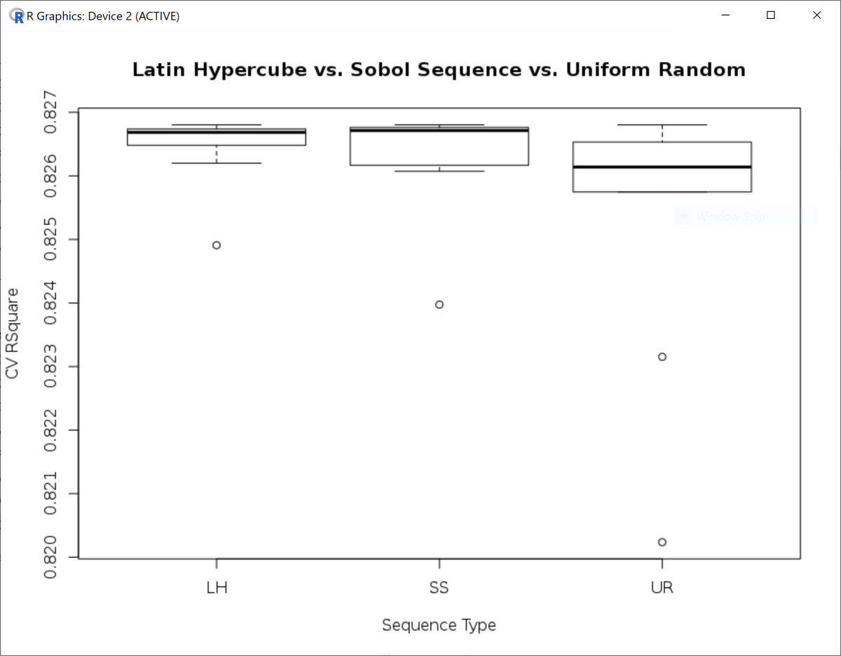
title <- "Latin Hypercube vs. Sobol Sequence vs. Uniform Random"
boxplot(R2 ~ type, data = out, main = title, ylab = "CV RSquare", xlab = "Sequence Type")

aggregate(R2 ~ type, data = out, function(x) round(c(avg = mean(x), var = var(x)), 8))
#type     R2.avg     R2.var
#  LH 0.82645414 0.00000033
#  SS 0.82632171 0.00000075
#  UR 0.82536693 0.00000432

Granular Weighted Binning by Generalized Boosted Model

In the post https://statcompute.wordpress.com/2019/04/27/more-general-weighted-binning, I’ve shown how to do the weighted binning with the function wqtl_bin() by the iterative partitioning. However, the outcome from wqtl_bin() sometimes can be too coarse. The function wgbm_bin() (https://github.com/statcompute/MonotonicBinning/blob/master/code/wgbm_bin.R) leverages the idea of gbm() that implements the Generalized Boosted Model and generates more granular weighted binning outcomes.

Below is the demonstration showing the difference between wqtl_bin() and wgbm_bin() outcomes. Even with the same data, the wgbm_bin() function is able to generate a more granular binning result and 14% higher Information Value.

	df <- readRDS("archive/accepts.rds")
	head(df, 1)
	# bankruptcy bad app_id tot_derog tot_tr age_oldest_tr tot_open_tr tot_rev_tr tot_rev_debt tot_rev_line rev_util bureau_score purch_price msrp
	# 0 0 1001 6 7 46 NaN NaN NaN NaN 0 747 19678 17160
	# down_pyt purpose loan_term loan_amt ltv tot_income used_ind weight
	# 947.15 LEASE 36 18730.85 109 4800 0 4.75
	### BY ITERATIVE PARTITION ###
	source("wqtl_bin.R")
	wqtl_bin(df, bad, tot_open_tr, weight)
	# bin rule cnt freq dist mv_wt bad_freq bad_rate woe iv ks
	# 00 is.na($X) 1416 5398.50 0.2323 5398.5 354 0.0656 0.2573 0.0173 6.7157
	# 01 $X <= 6 2994 12050.25 0.5185 0.0 579 0.0480 -0.0722 0.0026 3.0908
	# 02 $X > 6 1427 5792.00 0.2492 0.0 263 0.0454 -0.1315 0.0041 0.0000
	### BY GENERALIZED BOOSTED MODEL ###
	source("wgbm_bin.R")
	wgbm_bin(df, bad, tot_open_tr, weight)
	# bin rule cnt freq dist mv_wt bad_freq bad_rate woe iv ks
	# 00 is.na($X) 1416 5398.50 0.2323 5398.5 354 0.0656 0.2573 0.0173 6.7157
	# 01 $X <= 2 525 2085.00 0.0897 0.0 109 0.0523 0.0166 0.0000 6.8658
	# 02 $X > 2 & $X <= 3 605 2408.75 0.1036 0.0 124 0.0515 0.0004 0.0000 6.8695
	# 03 $X > 3 & $X <= 5 1319 5342.75 0.2299 0.0 246 0.0460 -0.1169 0.0030 4.3181
	# 04 $X > 5 & $X <= 14 1899 7696.50 0.3312 0.0 353 0.0459 -0.1210 0.0046 0.5213
	# 05 $X > 14 73 309.25 0.0133 0.0 10 0.0323 -0.4846 0.0025 0.0000

view raw

use_wtwoe.R

hosted with ❤ by GitHub

Batch Deployment of WoE Transformations

After wrapping up the function batch_woe() today with the purpose to allow users to apply WoE transformations to many independent variables simultaneously, I have completed the development of major functions in the MOB package that can be usable for the model development in a production setting.

The function batch_woe() basically is the wrapper around cal_woe() and has two input parameters. The “data” parameter is the data frame that we would deploy binning outcomes and the “slst” parameter is the list of multiple binning specification tables that is either the direct output from the function batch_bin or created manually by combining outputs from multiple binning functions.

There are also two components in the output of batch_woe(), a list of PSI tables for transformed variables and a data frame with a row index and all transformed variables. The default printout is a PSI summation of all input variables to be transformed. As shown below, all PSI values are below 0.1 and therefore none is concerning.

binout <- batch_bin(df, 1)

woeout <- batch_woe(df[sample(seq(nrow(df)), 2000, replace = T), ], binout$BinLst)

woeout 
#     tot_derog tot_tr age_oldest_tr tot_open_tr tot_rev_tr tot_rev_debt ...
# psi    0.0027 0.0044        0.0144      0.0011      3e-04       0.0013 ...

str(woeout, max.level = 1)
# List of 2
#  $ psi:List of 11
#  $ df :'data.frame':	2000 obs. of  12 variables:
#  - attr(*, "class")= chr "psiSummary"

head(woeout$df, 1)
#  idx_ woe.tot_derog woe.tot_tr woe.age_oldest_tr woe.tot_open_tr woe.tot_rev_tr ...
#     1       -0.3811    -0.0215           -0.5356         -0.0722        -0.1012 ...

All source codes of the MOB package are available on https://github.com/statcompute/MonotonicBinning and free (as free beer) to download and distribute.

Batch Processing of Monotonic Binning

In my GitHub repository (https://github.com/statcompute/MonotonicBinning), multiple R functions have been developed to implement the monotonic binning by using either iterative discretization or isotonic regression. With these functions, we can run the monotonic binning for one independent variable at a time. However, in a real-world production environment, we often would want to apply the binning algorithm to hundreds or thousands of variables at once. In addition, we might be interested in comparing different binning outcomes.

The function batch_bin() is designed to apply a monotonic binning function to all numeric variables in a data frame with the last column as the dependent variable. Currently, four binning algorithms are supported, including qtl_bin() and bad_bin() by iterative discretizations, iso_bin() by isotonic regression, and gbm_bin() by generalized boosted model. Before using these four functions, we need to save related R files in the working folder, which would be sourced by the batch_bin() function. Scripts for R functions can be downloaded from https://github.com/statcompute/MonotonicBinning/tree/master/code.

Below is the demonstrating showing how to use the batch_bin() function, which only requires two input parameters, a data frame and an integer number indicating the binning method. With method = 1, the batch_bin() function implements the iterative discretization by quantiles. With method = 4, the batch_bin() function implements the generalized boosted modelling. As shown below, both KS and IV with method = 4 are higher than with method = 1 due to more granular bins. For instance, while the method = 1 only generates 2 bins, the method = 4 can generate 11 bins.

	head(df, 2)
	# tot_derog tot_tr age_oldest_tr tot_open_tr tot_rev_tr tot_rev_debt tot_rev_line rev_util bureau_score ltv tot_income bad
	#1 6 7 46 NaN NaN NaN NaN 0 747 109 4800.00 0
	#2 0 21 153 6 1 97 4637 2 744 97 5833.33 0
	batch_bin(df, 1)
	#|var | nbin| unique| miss| min| median| max| ks| iv|
	#|:————–|—–:|——-:|—–:|—-:|——–:|——–:|——–:|——-:|
	#|tot_derog | 5| 29| 213| 0| 0.0| 32| 18.9469| 0.2055|
	#|tot_tr | 5| 67| 213| 0| 16.0| 77| 15.7052| 0.1302|
	#|age_oldest_tr | 10| 460| 216| 1| 137.0| 588| 19.9821| 0.2539|
	#|tot_open_tr | 3| 26| 1416| 0| 5.0| 26| 6.7157| 0.0240|
	#|tot_rev_tr | 3| 21| 636| 0| 3.0| 24| 9.0104| 0.0717|
	#|tot_rev_debt | 3| 3880| 477| 0| 3009.5| 96260| 8.5102| 0.0627|
	#|tot_rev_line | 9| 3617| 477| 0| 10573.0| 205395| 26.4924| 0.4077|
	#|rev_util | 2| 101| 0| 0| 30.0| 100| 15.1570| 0.0930|
	#|bureau_score | 12| 315| 315| 443| 692.5| 848| 34.8028| 0.7785|
	#|ltv | 7| 145| 1| 0| 100.0| 176| 15.6254| 0.1538|
	#|tot_income | 4| 1639| 5| 0| 3400.0| 8147167| 9.1526| 0.0500|
	batch_bin(df, 1)$BinLst[["rev_util"]]$df
	# bin rule freq dist mv_cnt bad_freq bad_rate woe iv ks
	# 01 $X <= 31 3007 0.5152 0 472 0.1570 -0.3250 0.0493 15.157
	# 02 $X > 31 2830 0.4848 0 724 0.2558 0.2882 0.0437 0.000
	batch_bin(df, 4)
	#|var | nbin| unique| miss| min| median| max| ks| iv|
	#|:————–|—–:|——-:|—–:|—-:|——–:|——–:|——–:|——-:|
	#|tot_derog | 8| 29| 213| 0| 0.0| 32| 20.0442| 0.2556|
	#|tot_tr | 13| 67| 213| 0| 16.0| 77| 17.3002| 0.1413|
	#|age_oldest_tr | 22| 460| 216| 1| 137.0| 588| 20.3646| 0.2701|
	#|tot_open_tr | 6| 26| 1416| 0| 5.0| 26| 6.8695| 0.0274|
	#|tot_rev_tr | 4| 21| 636| 0| 3.0| 24| 9.0779| 0.0789|
	#|tot_rev_debt | 9| 3880| 477| 0| 3009.5| 96260| 8.8722| 0.0848|
	#|tot_rev_line | 21| 3617| 477| 0| 10573.0| 205395| 26.8943| 0.4445|
	#|rev_util | 11| 101| 0| 0| 30.0| 100| 16.9615| 0.1635|
	#|bureau_score | 30| 315| 315| 443| 692.5| 848| 35.2651| 0.8344|
	#|ltv | 17| 145| 1| 0| 100.0| 176| 16.8807| 0.1911|
	#|tot_income | 17| 1639| 5| 0| 3400.0| 8147167| 10.3386| 0.0775|
	batch_bin(df, 4)$BinLst[["rev_util"]]$df
	# bin rule freq dist mv_cnt bad_freq bad_rate woe iv ks
	# 01 $X <= 24 2653 0.4545 0 414 0.1560 -0.3320 0.0452 13.6285
	# 02 $X > 24 & $X <= 36 597 0.1023 0 96 0.1608 -0.2963 0.0082 16.3969
	# 03 $X > 36 & $X <= 40 182 0.0312 0 32 0.1758 -0.1890 0.0011 16.9533
	# 04 $X > 40 & $X <= 58 669 0.1146 0 137 0.2048 -0.0007 0.0000 16.9615
	# 05 $X > 58 & $X <= 60 77 0.0132 0 16 0.2078 0.0177 0.0000 16.9381
	# 06 $X > 60 & $X <= 73 442 0.0757 0 103 0.2330 0.1647 0.0022 15.6305
	# 07 $X > 73 & $X <= 75 62 0.0106 0 16 0.2581 0.2999 0.0010 15.2839
	# 08 $X > 75 & $X <= 83 246 0.0421 0 70 0.2846 0.4340 0.0089 13.2233
	# 09 $X > 83 & $X <= 96 376 0.0644 0 116 0.3085 0.5489 0.0225 9.1266
	# 10 $X > 96 & $X <= 98 50 0.0086 0 17 0.3400 0.6927 0.0049 8.4162
	# 11 $X > 98 483 0.0827 0 179 0.3706 0.8263 0.0695 0.0000

view raw

use_BatchBin.R

hosted with ❤ by GitHub

Bayesian Optimization for Hyper-Parameter

In past several weeks, I spent a tremendous amount of time on reading literature about automatic parameter tuning in the context of Machine Learning (ML), most of which can be classified into two major categories, e.g. search and optimization. Searching mechanisms, such as grid search, random search, and Sobol sequence, can be somewhat computationally expensive. However, they are extremely easy to implement and parallelize on a multi-core PC, as shown in https://statcompute.wordpress.com/2019/02/03/sobol-sequence-vs-uniform-random-in-hyper-parameter-optimization. On the other hand, optimization algorithms, especially gradient-free optimizers such as Nelder–Mead simplex and particle swarm, are often able to quickly locate close-to-optimal solutions in cases that the global optimal is neither feasible nor necessary, as shown in https://statcompute.wordpress.com/2019/02/10/direct-optimization-of-hyper-parameter and https://statcompute.wordpress.com/2019/02/23/gradient-free-optimization-for-glmnet-parameters.

In the example below, another interesting approach, namely Bayesian optimization (https://arxiv.org/abs/1206.2944), is demonstrated and compared with CMA-ES (https://www.researchgate.net/publication/227050324_The_CMA_Evolution_Strategy_A_Comparing_Review), which is also a popular gradient-free optimizer based on the evolution strategy. As shown in the result, the output from Bayesian optimization is closer to the one from Nelder–Mead simplex and particle swarm. What’s more, Bayesian optimization is more consistent than CMA-ES among multiple trials in the experiment.

	cma_out <- cmaes::cma_es(
	par = 0.5,
	fn = function(x) grnn.optim(x, net, 4, 2019),
	lower = 0.1, upper = 1,
	control = list(fnscale = -1, mu = 20, lambda = 50))
	#$par
	#[1] 0.5766267
	#$value
	#[1] 0.8018076
	bay_out <- rBayesianOptimization::BayesianOptimization(
	FUN = function(x) list(Score = grnn.optim(x, net, 4, 2019), Pred = 0),
	bounds = list(x = c(0.1, 1)),
	init_points = 5, n_iter = 20,
	acq = "ucb", verbose = F)
	# Best Parameters Found:
	#Round = 20 x = 0.5583 Value = 0.8019

view raw

BayesianOptimization_GRNN.R

hosted with ❤ by GitHub

Direct Optimization of Hyper-Parameter

In the previous post (https://statcompute.wordpress.com/2019/02/03/sobol-sequence-vs-uniform-random-in-hyper-parameter-optimization), it is shown how to identify the optimal hyper-parameter in a General Regression Neural Network by using the Sobol sequence and the uniform random generator respectively through the N-fold cross validation. While the Sobol sequence yields a slightly better performance, outcomes from both approaches are very similar, as shown below based upon five trials with 20 samples in each. Both approaches can be generalized from one-dimensional to multi-dimensional domains, e.g. boosting or deep learning.

net <- grnn.fit(scale(Boston[, -14]), Boston[, 14], sigma = 1)
                        
sb_out <- Reduce(rbind, Map(function(x) grnn.cv(net, gen_sobol(0.1, 1.0, 20, x), 4, 2019), seq(1, 5)))

uf_out <- Reduce(rbind, Map(function(x) grnn.cv(net, gen_unifm(0.1, 1.0, 20, x), 4, 2019), seq(1, 5)))

Map(function(x) x[x$R2 == max(x$R2), ], list(sobol = sb_out, uniform = uf_out))
# $sobol
#  sigma        R2
# 0.5568 0.8019342
# $uniform
#  sigma        R2
# 0.5608 0.8019327

Other than the random search, another way to locate the optimal hyper-parameter is applying general optimization routines, As shown in the demonstration below, we first need to define an objective function, e.g. grnn.optim(), to maximize the Cross-Validation R^2. In addition, depending on the optimization algorithm, upper and lower bounds of the parameter to be optimized should also be provided. Three optimization algorithms are employed in the example, including unconstrained non-linear optimization, particle swarm optimization, and Nelder–Mead simplex optimization, with all showing comparable outcomes to ones achieved by the random search.

	net <- grnn.fit(scale(Boston[, -14]), Boston[, 14], sigma = 1)
	grnn.optim <- function(sigma, nn, nfolds, seed) {
	dt <- nn$set
	set.seed(seed)
	folds <- caret::createFolds(1:nrow(dt), k = nfolds, list = FALSE)
	r <- do.call(rbind,
	lapply(1:nfolds,
	function(i) data.frame(Ya = nn$Ya[folds == i],
	Yp = grnn.predict(grnn.fit(nn$Xa[folds != i, ], nn$Ya[folds != i], sigma),
	data.frame(nn$Xa[folds == i,])))))
	return(r2(r$Ya, r$Yp))
	}
	### General-Purpose Unconstrained Non-Linear Optimization ###
	op_out <- ucminf::ucminf(par = 0.5, fn = function(x) -grnn.optim(x, net, 4, 2019))
	# $par
	# [1] 0.5611872
	# $value
	# [1] -0.8019319
	### Particle Swarm Optimization ###
	set.seed(1)
	ps_out <- pso::psoptim(par = 0.5, upper = 1.0, lower = 0.1,
	fn = function(x) -grnn.optim(x, net, 4, 2019),
	control = list(maxit = 20))
	# $par
	# [1] 0.5583358
	# $value
	# [1] -0.8019351
	### Nelder–Mead Optimization ###
	nm_out <- optim(par = 0.5, fn = function(x) -grnn.optim(x, net, 4, 2019),
	method = "Nelder-Mead", control = list(warn.1d.NelderMead = FALSE))
	# $par
	# [1] 0.5582031
	# $value
	# [1] -0.8019351

view raw

grnn_optim.R

hosted with ❤ by GitHub

Sobol Sequence vs. Uniform Random in Hyper-Parameter Optimization

Tuning hyper-parameters might be the most tedious yet crucial in various machine learning algorithms, such as neural networks, svm, or boosting. The configuration of hyper-parameters not only impacts the computational efficiency of a learning algorithm but also determines its prediction accuracy.

Thus far, manual tuning and grid searching are still the most prevailing strategies. In the paper http://www.jmlr.org/papers/volume13/bergstra12a/bergstra12a.pdf, Bergstra and Bengio showed that the random search is more efficient in the hyper-parameter optimization than both the grid search and the manual tuning. Following the similar logic of the random search, a Sobol sequence is a series of quasi-random numbers designed to cover the space more evenly than uniform random numbers.

The demonstration below compared the Sobol sequence and the uniform random number generator in the hyper-parameter tuning of a General Regression Neural Network (GRNN). In this particular example, the Sobol sequence outperforms the uniform random number generator in two folds. First of all, it picks the hyper-parameter that yields a better performance, e.g. R^2, in the cross-validation. Secondly, the performance is more consistent in multiple trials with a lower variance.

	data(Boston, package = "MASS")
	grnn.fit <- function(x, y, sigma) {
	return(grnn::smooth(grnn::learn(data.frame(y, x)), sigma))
	}
	grnn.predict <- function(nn, x) {
	c <- parallel::detectCores() – 1
	return(do.call(rbind,
	parallel::mcMap(function(i) grnn::guess(nn, as.matrix(x[i, ])),
	1:nrow(x), mc.cores = c))[,1])
	}
	r2 <- function(act, pre) {
	rss <- sum((pre – act) ^ 2)
	tss <- sum((act – mean(act)) ^ 2)
	return(1 – rss / tss)
	}
	grnn.cv <- function(nn, sigmas, nfolds, seed) {
	dt <- nn$set
	set.seed(seed)
	folds <- caret::createFolds(1:nrow(dt), k = nfolds, list = FALSE)
	cv <- function(s) {
	r <- do.call(rbind,
	lapply(1:nfolds,
	function(i) data.frame(Ya = nn$Ya[folds == i],
	Yp = grnn.predict(grnn.fit(nn$Xa[folds != i, ], nn$Ya[folds != i], s),
	data.frame(nn$Xa[folds == i,])))))
	return(data.frame(sigma = s, R2 = r2(r$Ya, r$Yp)))
	}
	r2_lst <- Reduce(rbind, Map(cv, sigmas))
	return(r2_lst[r2_lst$R2 == max(r2_lst$R2), ])
	}
	gen_sobol <- function(min, max, n, seed) {
	return(round(min + (max – min) * randtoolbox::sobol(n, dim = 1, scrambling = 1, seed = seed), 4))
	}
	gen_unifm <- function(min, max, n, seed) {
	set.seed(seed)
	return(round(min + (max – min) * runif(n), 4))
	}
	net <- grnn.fit(Boston[, -14], Boston[, 14], sigma = 2)
	sobol_out <- Reduce(rbind, Map(function(x) grnn.cv(net, gen_sobol(5, 10, 10, x), 4, 2019), seq(1, 10)))
	unifm_out <- Reduce(rbind, Map(function(x) grnn.cv(net, gen_unifm(5, 10, 10, x), 4, 2019), seq(1, 10)))
	out <- rbind(cbind(type = rep("sobol", 10), sobol_out),
	cbind(type = rep("unifm", 10), unifm_out))
	boxplot(R2 ~ type, data = out, main = "Sobol Sequence vs. Uniform Random",
	ylab = "CV RSquare", xlab = "Sequence Type")

view raw

sobol_grnn.R

hosted with ❤ by GitHub

Adding New Columns to Clojure Map

(require '[huri.core :as h]
         '[clojure.core.matrix.dataset :as d]
         '[incanter.core :as i])

(def ds [{:id 1.0 :name "name1"}
         {:id 2.0 :name "name2"}
         {:id 3.0 :name "name3"}])

;; ADD 2 COLUMNS TO THE DATASET
;; - ADD 2 TO ID AND NAME ADD2
;; - CHECK NAME = "name2" AND NAME NAME2
;;
;; EXPECTED OUTPUT:
;;| :id | :name | :add2 | :name2 |
;;|-----+-------+-------+--------|
;;| 1.0 | name1 |   3.0 |      N |
;;| 2.0 | name2 |   4.0 |      Y |
;;| 3.0 | name3 |   5.0 |      N |

;; WITH PLAIN CLOJURE
;; #1 - MERGE
(def d1 (map #(merge % {:add2 (+ (:id %) 2) 
                        :name2 (if (= "name2" (:name %)) "Y" "N")}) ds))

;; #2 - MERGE-WITH
(def d2 (map #(merge-with into % {:add2 (+ (:id %) 2)
                                  :name2 (if (= "name2" (:name %)) "Y" "N")}) ds))

;; #3 - ASSOC
(def d3 (map #(assoc % :add2 (+ (:id %) 2) 
                       :name2 (if (= "name2" (:name %)) "Y" "N")) ds))

;; #4 - CONJ
(def d4 (map #(conj % {:add2 (+ (:id %) 2)
                       :name2 (if (= "name2" (:name %)) "Y" "N")}) ds))

;; #5 - CONCAT 
(def d5 (map #(into {} (concat % {:add2 (+ (:id %) 2)
                                  :name2 (if (= "name2" (:name %)) "Y" "N")})) ds))

;; WITH HURI 
(def d6 (h/derive-cols {:name2 [#(if (= "name2" %) "Y" "N") :name] 
                        :add2 [#(+ 2  %) :id]} ds))

;; WITH CORE.MATRIX API
(def d7 (-> ds
            (d/dataset)
            (d/add-column :add2 (map #(+ 2 %) (map :id ds)))
            (d/add-column :name2 (map #(if (= "name2" %) "Y" "N") (map :name ds)))
            (d/row-maps)))

;; WITH INCANTER API
(def d8 (->> ds
             (i/to-dataset)
             (i/add-derived-column :add2 [:id] #(+ 2 %))
             (i/add-derived-column :name2 [:name] #(if (= "name2" %) "Y" "N"))
             ((comp second vals))))

;; CHECK THE DATA EQUALITY
(= d1 d2 d3 d4 d5 d6 d7 d8)
;; true

Variable Selection with Elastic Net

LASSO has been a popular algorithm for the variable selection and extremely effective with high-dimension data. However, it often tends to “over-regularize” a model that might be overly compact and therefore under-predictive.

The Elastic Net addresses the aforementioned “over-regularization” by balancing between LASSO and ridge penalties. In particular, a hyper-parameter, namely Alpha, would be used to regularize the model such that the model would become a LASSO in case of Alpha = 1 and a ridge in case of Alpha = 0. In practice, Alpha can be tuned easily by the cross-validation. Below is a demonstration of Elastic Net with R glmnet package and its comparison with LASSO and ridge models.

pkgs <- list("glmnet", "doParallel", "foreach", "pROC")
lapply(pkgs, require, character.only = T)
registerDoParallel(cores = 4)
 
df1 <- read.csv("Downloads/credit_count.txt")
df2 <- df1[df1$CARDHLDR == 1, ]
set.seed(2017)
n <- nrow(df2)
sample <- sample(seq(n), size = n * 0.5, replace = FALSE)
train <- df2[sample, -1]
test <- df2[-sample, -1]
mdlY <- as.factor(as.matrix(train["DEFAULT"]))
mdlX <- as.matrix(train[setdiff(colnames(df1), c("CARDHLDR", "DEFAULT"))])
newY <- as.factor(as.matrix(test["DEFAULT"]))
newX <- as.matrix(test[setdiff(colnames(df1), c("CARDHLDR", "DEFAULT"))])

First of all, we estimates a LASSO model with Alpha = 1. The function cv.glmnet() is used to search for a regularization parameter, namely Lambda, that controls the penalty strength. As shown below, the model only identifies 2 attributes out of total 12.

# LASSO WITH ALPHA = 1
cv1 <- cv.glmnet(mdlX, mdlY, family = "binomial", nfold = 10, type.measure = "deviance", paralle = TRUE, alpha = 1)
md1 <- glmnet(mdlX, mdlY, family = "binomial", lambda = cv1$lambda.1se, alpha = 1)
coef(md1)
#(Intercept) -1.963030e+00
#AGE          .           
#ACADMOS      .           
#ADEPCNT      .           
#MAJORDRG     .           
#MINORDRG     .           
#OWNRENT      .           
#INCOME      -5.845981e-05
#SELFEMPL     .           
#INCPER       .           
#EXP_INC      .           
#SPENDING     .           
#LOGSPEND    -4.015902e-02
roc(newY, as.numeric(predict(md1, newX, type = "response")))
#Area under the curve: 0.636

We next estimates a ridge model as below by setting Alpha = 0. Similarly, Lambda is searched by the cross-validation. Since the ridge penalty would only regularize the magnitude of each coefficient, we end up with a “full” model with all model attributes. The model performance is slightly better with 10 more variables, which is a debatable outcome.

# RIDGE WITH ALPHA = 0
cv2 <- cv.glmnet(mdlX, mdlY, family = "binomial", nfold = 10, type.measure = "deviance", paralle = TRUE, alpha = 0)
md2 <- glmnet(mdlX, mdlY, family = "binomial", lambda = cv2$lambda.1se, alpha = 0)
coef(md2)
#(Intercept) -2.221016e+00
#AGE         -4.184422e-04
#ACADMOS     -3.085096e-05
#ADEPCNT      1.485114e-04
#MAJORDRG     6.684849e-03
#MINORDRG     1.006660e-03
#OWNRENT     -9.082750e-03
#INCOME      -6.960253e-06
#SELFEMPL     3.610381e-03
#INCPER      -3.881890e-07
#EXP_INC     -1.416971e-02
#SPENDING    -1.638184e-05
#LOGSPEND    -6.213884e-03
roc(newY, as.numeric(predict(md2, newX, type = "response")))
#Area under the curve: 0.6435

At last, we use the Elastic Net by tuning the value of Alpha through a line search with the parallelism. In this particular case, Alpha = 0.3 is chosen through the cross-validation. As shown below, 6 variables are used in the model that even performs better than the ridge model with all 12 attributes.

# ELASTIC NET WITH 0 < ALPHA < 1
a <- seq(0.1, 0.9, 0.05)
search <- foreach(i = a, .combine = rbind) %dopar% {
  cv <- cv.glmnet(mdlX, mdlY, family = "binomial", nfold = 10, type.measure = "deviance", paralle = TRUE, alpha = i)
  data.frame(cvm = cv$cvm[cv$lambda == cv$lambda.1se], lambda.1se = cv$lambda.1se, alpha = i)
}
cv3 <- search[search$cvm == min(search$cvm), ]
md3 <- glmnet(mdlX, mdlY, family = "binomial", lambda = cv3$lambda.1se, alpha = cv3$alpha)
coef(md3)
#(Intercept) -1.434700e+00
#AGE         -8.426525e-04
#ACADMOS      .           
#ADEPCNT      .           
#MAJORDRG     6.276924e-02
#MINORDRG     .           
#OWNRENT     -2.780958e-02
#INCOME      -1.305118e-04
#SELFEMPL     .           
#INCPER      -2.085349e-06
#EXP_INC      .           
#SPENDING     .           
#LOGSPEND    -9.992808e-02
roc(newY, as.numeric(predict(md3, newX, type = "response")))
#Area under the curve: 0.6449

DART: Dropout Regularization in Boosting Ensembles

The dropout approach developed by Hinton has been widely employed in deep learnings to prevent the deep neural network from overfitting, as shown in https://statcompute.wordpress.com/2017/01/02/dropout-regularization-in-deep-neural-networks.

In the paper http://proceedings.mlr.press/v38/korlakaivinayak15.pdf, the dropout can also be used to address the overfitting in boosting tree ensembles, e.g. MART, caused by the so-called “over-specialization”. In particular, while first few trees added at the beginning of ensembles would dominate the model performance, the rest added later can only improve the prediction for a small subset, which increases the risk of overfitting. The idea of DART is to build an ensemble by randomly dropping boosting tree members. The percentage of dropouts can determine the degree of regularization for boosting tree ensembles.

Below is a demonstration showing the implementation of DART with the R xgboost package. First of all, after importing the data, we divided it into two pieces, one for training and the other for testing.

pkgs <- c('pROC', 'xgboost')
lapply(pkgs, require, character.only = T)
df1 <- read.csv("Downloads/credit_count.txt")
df2 <- df1[df1$CARDHLDR == 1, ]
set.seed(2017)
n <- nrow(df2)
sample <- sample(seq(n), size = n / 2, replace = FALSE)
train <- df2[sample, -1]
test <- df2[-sample, -1]

For the comparison purpose, we first developed a boosting tree ensemble without dropouts, as shown below. For the simplicity, all parameters were chosen heuristically. The max_depth is set to 3 due to the fact that the boosting tends to work well with so-called “weak” learners, e.g. simple trees. While ROC for the training set can be as high as 0.95, ROC for the testing set is only 0.60 in our case, implying the overfitting issue.

mart.parm <- list(booster = "gbtree", nthread = 4, eta = 0.1, max_depth = 3, subsample = 1, eval_metric = "auc")
mart <- xgboost(data = as.matrix(train[, -1]), label = train[, 1], params = mart.parm, nrounds = 500, verbose = 0, seed = 2017)
pred1 <- predict(mart, as.matrix(train[, -1]))
pred2 <- predict(mart, as.matrix(test[, -1]))
roc(as.factor(train$DEFAULT), pred1)
# Area under the curve: 0.9459
roc(as.factor(test$DEFAULT), pred2)
# Area under the curve: 0.6046

With the same set of parameters, we refitted the ensemble with dropouts, e.g. DART. As shown below, by dropping 10% tree members, ROC for the testing set can increase from 0.60 to 0.65. In addition, the performance disparity between training and testing sets with DART decreases significantly.

dart.parm <- list(booster = "dart", rate_drop = 0.1, nthread = 4, eta = 0.1, max_depth = 3, subsample = 1, eval_metric = "auc")
dart <- xgboost(data = as.matrix(train[, -1]), label = train[, 1], params = dart.parm, nrounds = 500, verbose = 0, seed = 2017)
pred1 <- predict(dart, as.matrix(train[, -1]))
pred2 <- predict(dart, as.matrix(test[, -1]))
roc(as.factor(train$DEFAULT), pred1)
# Area under the curve: 0.7734
roc(as.factor(test$DEFAULT), pred2)
# Area under the curve: 0.6517

Besides rate_drop = 0.1, a wide range of dropout rates have also been tested. In most cases, DART outperforms its counterpart without the dropout regularization.

GLM with H2O in R

Below is an example showing how to fit a Generalized Linear Model with H2O in R. The output is much more comprehensive than the one generated by the generic R glm().

> library(h2o)

> h2o.init(max_mem_size = "12g")

> df1 <- h2o.uploadFile("Documents/credit_count.txt", header = TRUE, sep = ",", parse_type = "CSV")

> df2 <- h2o.assign(df1[df1$CARDHLDR == 1, ], "glm_df")

> h2o.colnames(df2)
 [1] "CARDHLDR" "DEFAULT"  "AGE"      "ACADMOS"  "ADEPCNT"  "MAJORDRG"
 [7] "MINORDRG" "OWNRENT"  "INCOME"   "SELFEMPL" "INCPER"   "EXP_INC"
[13] "SPENDING" "LOGSPEND"

> Y <- "DEFAULT"

> X <- c("MAJORDRG", "MINORDRG", "INCOME", "OWNRENT")

> dist <- "binomial"

> link <- "logit"

> id <- "h2o_mdl01"

> mdl <- h2o.glm(X, Y, training_frame = h2o.getFrame("glm_df"), model_id = id, family = dist, link = link, lambda = 0, compute_p_values = TRUE, standardize = FALSE)

> show(h2o.getModel(id)@model$coefficients_table)
Coefficients: glm coefficients
      names coefficients std_error    z_value  p_value
1 Intercept    -1.204439  0.090811 -13.263121 0.000000
2  MAJORDRG     0.203135  0.069250   2.933370 0.003353
3  MINORDRG     0.202727  0.047971   4.226014 0.000024
4   OWNRENT    -0.201223  0.071619  -2.809636 0.004960
5    INCOME    -0.000442  0.000040 -10.942350 0.000000

> h2o.performance(h2o.getModel(id))
H2OBinomialMetrics: glm
** Reported on training data. **

MSE:  0.08414496
RMSE:  0.2900775
LogLoss:  0.3036585
Mean Per-Class Error:  0.410972
AUC:  0.6432189
Gini:  0.2864378
R^2:  0.02005004
Residual Deviance:  6376.221
AIC:  6386.221

Confusion Matrix (vertical: actual; across: predicted) for F1-optimal threshold:
          0    1    Error         Rate
0      7703 1800 0.189414   =1800/9503
1       630  366 0.632530     =630/996
Totals 8333 2166 0.231451  =2430/10499

Maximum Metrics: Maximum metrics at their respective thresholds
                        metric threshold    value idx
1                       max f1  0.126755 0.231499 142
2                       max f2  0.075073 0.376556 272
3                 max f0point5  0.138125 0.191828 115
4                 max accuracy  0.368431 0.905039   0
5                max precision  0.314224 0.250000   3
6                   max recall  0.006115 1.000000 399
7              max specificity  0.368431 0.999895   0
8             max absolute_mcc  0.126755 0.128940 142
9   max min_per_class_accuracy  0.106204 0.604546 196
10 max mean_per_class_accuracy  0.103730 0.605663 202

Finer Monotonic Binning Based on Isotonic Regression

In my early post (https://statcompute.wordpress.com/2017/01/22/monotonic-binning-with-smbinning-package/), I wrote a monobin() function based on the smbinning package by Herman Jopia to improve the monotonic binning algorithm. The function works well and provides robust binning outcomes. However, there are a couple potential drawbacks due to the coarse binning. First of all, the derived Information Value for each binned variable might tend to be low. Secondly, the binned variable might not be granular enough to reflect the data nature.

In light of the aforementioned, I drafted an improved function isobin() based on the isotonic regression (https://en.wikipedia.org/wiki/Isotonic_regression), as shown below.

isobin <- function(data, y, x) {
  d1 <- data[c(y, x)]
  d2 <- d1[!is.na(d1[x]), ]
  c <- cor(d2[, 2], d2[, 1], method = "spearman", use = "complete.obs")
  reg <- isoreg(d2[, 2], c / abs(c) * d2[, 1])
  k <- knots(as.stepfun(reg))
  sm1 <-smbinning.custom(d1, y, x, k)
  c1 <- subset(sm1$ivtable, subset = CntGood * CntBad > 0, select = Cutpoint)
  c2 <- suppressWarnings(as.numeric(unlist(strsplit(c1$Cutpoint, " "))))
  c3 <- c2[!is.na(c2)]
  return(smbinning.custom(d1, y, x, c3[-length(c3)]))
}

Compared with the legacy monobin(), the isobin() function is able to significantly increase the binning granularity as well as moderately improve the Information Value.

LTV Binning with isobin() Function

   Cutpoint CntRec CntGood CntBad CntCumRec CntCumGood CntCumBad PctRec GoodRate BadRate    Odds LnOdds     WoE     IV
1     <= 46     81      78      3        81         78         3 0.0139   0.9630  0.0370 26.0000 3.2581  1.9021 0.0272
2     <= 71    312     284     28       393        362        31 0.0535   0.9103  0.0897 10.1429 2.3168  0.9608 0.0363
3     <= 72     22      20      2       415        382        33 0.0038   0.9091  0.0909 10.0000 2.3026  0.9466 0.0025
4     <= 73     27      24      3       442        406        36 0.0046   0.8889  0.1111  8.0000 2.0794  0.7235 0.0019
5     <= 81    303     268     35       745        674        71 0.0519   0.8845  0.1155  7.6571 2.0356  0.6797 0.0194
6     <= 83    139     122     17       884        796        88 0.0238   0.8777  0.1223  7.1765 1.9708  0.6149 0.0074
7     <= 90    631     546     85      1515       1342       173 0.1081   0.8653  0.1347  6.4235 1.8600  0.5040 0.0235
8     <= 94    529     440     89      2044       1782       262 0.0906   0.8318  0.1682  4.9438 1.5981  0.2422 0.0049
9     <= 95    145     119     26      2189       1901       288 0.0248   0.8207  0.1793  4.5769 1.5210  0.1651 0.0006
10   <= 100    907     709    198      3096       2610       486 0.1554   0.7817  0.2183  3.5808 1.2756 -0.0804 0.0010
11   <= 101    195     151     44      3291       2761       530 0.0334   0.7744  0.2256  3.4318 1.2331 -0.1229 0.0005
12   <= 110   1217     934    283      4508       3695       813 0.2085   0.7675  0.2325  3.3004 1.1940 -0.1619 0.0057
13   <= 112    208     158     50      4716       3853       863 0.0356   0.7596  0.2404  3.1600 1.1506 -0.2054 0.0016
14   <= 115    253     183     70      4969       4036       933 0.0433   0.7233  0.2767  2.6143 0.9610 -0.3950 0.0075
15   <= 136    774     548    226      5743       4584      1159 0.1326   0.7080  0.2920  2.4248 0.8857 -0.4702 0.0333
16   <= 138     27      18      9      5770       4602      1168 0.0046   0.6667  0.3333  2.0000 0.6931 -0.6628 0.0024
17    > 138     66      39     27      5836       4641      1195 0.0113   0.5909  0.4091  1.4444 0.3677 -0.9882 0.0140
18  Missing      1       0      1      5837       4641      1196 0.0002   0.0000  1.0000  0.0000   -Inf    -Inf    Inf
19    Total   5837    4641   1196        NA         NA        NA 1.0000   0.7951  0.2049  3.8804 1.3559  0.0000 0.1897

LTV Binning with monobin() Function

  Cutpoint CntRec CntGood CntBad CntCumRec CntCumGood CntCumBad PctRec GoodRate BadRate   Odds LnOdds     WoE     IV
1    <= 85   1025     916    109      1025        916       109 0.1756   0.8937  0.1063 8.4037 2.1287  0.7727 0.0821
2    <= 94   1019     866    153      2044       1782       262 0.1746   0.8499  0.1501 5.6601 1.7334  0.3775 0.0221
3   <= 100   1052     828    224      3096       2610       486 0.1802   0.7871  0.2129 3.6964 1.3074 -0.0486 0.0004
4   <= 105    808     618    190      3904       3228       676 0.1384   0.7649  0.2351 3.2526 1.1795 -0.1765 0.0045
5   <= 114    985     748    237      4889       3976       913 0.1688   0.7594  0.2406 3.1561 1.1493 -0.2066 0.0076
6    > 114    947     665    282      5836       4641      1195 0.1622   0.7022  0.2978 2.3582 0.8579 -0.4981 0.0461
7  Missing      1       0      1      5837       4641      1196 0.0002   0.0000  1.0000 0.0000   -Inf    -Inf    Inf
8    Total   5837    4641   1196        NA         NA        NA 1.0000   0.7951  0.2049 3.8804 1.3559  0.0000 0.1628

Bureau_Score Binning with isobin() Function

   Cutpoint CntRec CntGood CntBad CntCumRec CntCumGood CntCumBad PctRec GoodRate BadRate    Odds  LnOdds     WoE     IV
1    <= 491      4       1      3         4          1         3 0.0007   0.2500  0.7500  0.3333 -1.0986 -2.4546 0.0056
2    <= 532     24       9     15        28         10        18 0.0041   0.3750  0.6250  0.6000 -0.5108 -1.8668 0.0198
3    <= 559     51      24     27        79         34        45 0.0087   0.4706  0.5294  0.8889 -0.1178 -1.4737 0.0256
4    <= 560      2       1      1        81         35        46 0.0003   0.5000  0.5000  1.0000  0.0000 -1.3559 0.0008
5    <= 572     34      17     17       115         52        63 0.0058   0.5000  0.5000  1.0000  0.0000 -1.3559 0.0143
6    <= 602    153      84     69       268        136       132 0.0262   0.5490  0.4510  1.2174  0.1967 -1.1592 0.0459
7    <= 605     56      31     25       324        167       157 0.0096   0.5536  0.4464  1.2400  0.2151 -1.1408 0.0162
8    <= 606     14       8      6       338        175       163 0.0024   0.5714  0.4286  1.3333  0.2877 -1.0683 0.0035
9    <= 607     17      10      7       355        185       170 0.0029   0.5882  0.4118  1.4286  0.3567 -0.9993 0.0037
10   <= 632    437     261    176       792        446       346 0.0749   0.5973  0.4027  1.4830  0.3940 -0.9619 0.0875
11   <= 639    150      95     55       942        541       401 0.0257   0.6333  0.3667  1.7273  0.5465 -0.8094 0.0207
12   <= 653    451     300    151      1393        841       552 0.0773   0.6652  0.3348  1.9868  0.6865 -0.6694 0.0412
13   <= 662    295     213     82      1688       1054       634 0.0505   0.7220  0.2780  2.5976  0.9546 -0.4014 0.0091
14   <= 665    100      77     23      1788       1131       657 0.0171   0.7700  0.2300  3.3478  1.2083 -0.1476 0.0004
15   <= 667     57      44     13      1845       1175       670 0.0098   0.7719  0.2281  3.3846  1.2192 -0.1367 0.0002
16   <= 677    381     300     81      2226       1475       751 0.0653   0.7874  0.2126  3.7037  1.3093 -0.0466 0.0001
17   <= 679     66      53     13      2292       1528       764 0.0113   0.8030  0.1970  4.0769  1.4053  0.0494 0.0000
18   <= 683    160     129     31      2452       1657       795 0.0274   0.8062  0.1938  4.1613  1.4258  0.0699 0.0001
19   <= 689    203     164     39      2655       1821       834 0.0348   0.8079  0.1921  4.2051  1.4363  0.0804 0.0002
20   <= 699    304     249     55      2959       2070       889 0.0521   0.8191  0.1809  4.5273  1.5101  0.1542 0.0012
21   <= 707    312     268     44      3271       2338       933 0.0535   0.8590  0.1410  6.0909  1.8068  0.4509 0.0094
22   <= 717    368     318     50      3639       2656       983 0.0630   0.8641  0.1359  6.3600  1.8500  0.4941 0.0132
23   <= 721    134     119     15      3773       2775       998 0.0230   0.8881  0.1119  7.9333  2.0711  0.7151 0.0094
24   <= 723     49      44      5      3822       2819      1003 0.0084   0.8980  0.1020  8.8000  2.1748  0.8188 0.0043
25   <= 739    425     394     31      4247       3213      1034 0.0728   0.9271  0.0729 12.7097  2.5424  1.1864 0.0700
26   <= 746    166     154     12      4413       3367      1046 0.0284   0.9277  0.0723 12.8333  2.5520  1.1961 0.0277
27   <= 756    234     218     16      4647       3585      1062 0.0401   0.9316  0.0684 13.6250  2.6119  1.2560 0.0422
28   <= 761    110     104      6      4757       3689      1068 0.0188   0.9455  0.0545 17.3333  2.8526  1.4967 0.0260
29   <= 763     46      44      2      4803       3733      1070 0.0079   0.9565  0.0435 22.0000  3.0910  1.7351 0.0135
30   <= 767     96      92      4      4899       3825      1074 0.0164   0.9583  0.0417 23.0000  3.1355  1.7795 0.0293
31   <= 772     77      74      3      4976       3899      1077 0.0132   0.9610  0.0390 24.6667  3.2055  1.8495 0.0249
32   <= 787    269     260      9      5245       4159      1086 0.0461   0.9665  0.0335 28.8889  3.3635  2.0075 0.0974
33   <= 794     95      93      2      5340       4252      1088 0.0163   0.9789  0.0211 46.5000  3.8395  2.4835 0.0456
34    > 794    182     179      3      5522       4431      1091 0.0312   0.9835  0.0165 59.6667  4.0888  2.7328 0.0985
35  Missing    315     210    105      5837       4641      1196 0.0540   0.6667  0.3333  2.0000  0.6931 -0.6628 0.0282
36    Total   5837    4641   1196        NA         NA        NA 1.0000   0.7951  0.2049  3.8804  1.3559  0.0000 0.8357

Bureau_Score Binning with monobin() Function

   Cutpoint CntRec CntGood CntBad CntCumRec CntCumGood CntCumBad PctRec GoodRate BadRate    Odds LnOdds     WoE     IV
1    <= 617    513     284    229       513        284       229 0.0879   0.5536  0.4464  1.2402 0.2153 -1.1407 0.1486
2    <= 642    515     317    198      1028        601       427 0.0882   0.6155  0.3845  1.6010 0.4706 -0.8853 0.0861
3    <= 657    512     349    163      1540        950       590 0.0877   0.6816  0.3184  2.1411 0.7613 -0.5946 0.0363
4    <= 672    487     371    116      2027       1321       706 0.0834   0.7618  0.2382  3.1983 1.1626 -0.1933 0.0033
5    <= 685    494     396     98      2521       1717       804 0.0846   0.8016  0.1984  4.0408 1.3964  0.0405 0.0001
6    <= 701    521     428     93      3042       2145       897 0.0893   0.8215  0.1785  4.6022 1.5265  0.1706 0.0025
7    <= 714    487     418     69      3529       2563       966 0.0834   0.8583  0.1417  6.0580 1.8014  0.4454 0.0144
8    <= 730    489     441     48      4018       3004      1014 0.0838   0.9018  0.0982  9.1875 2.2178  0.8619 0.0473
9    <= 751    513     476     37      4531       3480      1051 0.0879   0.9279  0.0721 12.8649 2.5545  1.1986 0.0859
10   <= 775    492     465     27      5023       3945      1078 0.0843   0.9451  0.0549 17.2222 2.8462  1.4903 0.1157
11    > 775    499     486     13      5522       4431      1091 0.0855   0.9739  0.0261 37.3846 3.6213  2.2653 0.2126
12  Missing    315     210    105      5837       4641      1196 0.0540   0.6667  0.3333  2.0000 0.6931 -0.6628 0.0282
13    Total   5837    4641   1196        NA         NA        NA 1.0000   0.7951  0.2049  3.8804 1.3559  0.0000 0.7810

Random Search for Optimal Parameters

Practices of manual search, grid search, or the combination of both have been successfully employed in the machine learning to optimize hyper-parameters. However, in the arena of deep learning, both approaches might become impractical. For instance, the computing cost of grid search for hyper-parameters in a multi-layer deep neural network (DNN) could be prohibitively high.

In light of aforementioned hurdles, Bergstra and Bengio proposed a novel idea of random search in the paper http://www.jmlr.org/papers/volume13/bergstra12a/bergstra12a.pdf. In their study, it was found that random search is more efficient than grid search for the hyper-parameter optimization in terms of computing costs.

In the example below, it is shown that both grid search and random search have reached similar results in the SVM parameter optimization based on cross-validations.

import pandas as pd
import numpy as np
from sklearn import preprocessing
from sklearn.model_selection import GridSearchCV, RandomizedSearchCV 
from sklearn.svm import SVC as svc 
from sklearn.metrics import make_scorer, roc_auc_score
from scipy import stats

# DATA PREPARATION
df = pd.read_csv("credit_count.txt")
y = df[df.CARDHLDR == 1].DEFAULT.values 
x = preprocessing.scale(df[df.CARDHLDR == 1].ix[:, 2:12], axis = 0) 

# DEFINE MODEL AND PERFORMANCE MEASURE
mdl = svc(probability = True, random_state = 1)
auc = make_scorer(roc_auc_score)

# GRID SEARCH FOR 20 COMBINATIONS OF PARAMETERS
grid_list = {"C": np.arange(2, 10, 2),
             "gamma": np.arange(0.1, 1, 0.2)}

grid_search = GridSearchCV(mdl, param_grid = grid_list, n_jobs = 4, cv = 3, scoring = auc) 
grid_search.fit(x, y) 
grid_search.cv_results_

# RANDOM SEARCH FOR 20 COMBINATIONS OF PARAMETERS
rand_list = {"C": stats.uniform(2, 10),
             "gamma": stats.uniform(0.1, 1)}
             
rand_search = RandomizedSearchCV(mdl, param_distributions = rand_list, n_iter = 20, n_jobs = 4, cv = 3, random_state = 2017, scoring = auc) 
rand_search.fit(x, y) 
rand_search.cv_results_

A Simple Convolutional Neural Network for The Binary Outcome

Since CNN(Convolutional Neural Networks) have achieved a tremendous success in various challenging applications, e.g. image or digit recognitions, one might wonder how to employ CNNs in classification problems with binary outcomes.

Below is an example showing how to use a simple 1D convolutional neural network to predict credit card defaults.

### LOAD PACKAGES 
from numpy.random import seed
from pandas import read_csv, DataFrame
from sklearn.preprocessing import minmax_scale
from keras.layers.convolutional import Conv1D, MaxPooling1D
from keras.optimizers import SGD
from keras.models import Sequential
from keras.layers import Dense, Flatten

### PREPARE THE DATA 
df = read_csv("credit_count.txt")
Y = df[df.CARDHLDR == 1].DEFAULT
X = minmax_scale(df[df.CARDHLDR == 1].ix[:, 2:12], axis = 0)
y_train = Y.values
x_train = X.reshape(X.shape[0], X.shape[1], 1)

### FIT A 1D CONVOLUTIONAL NEURAL NETWORK
seed(2017)
conv = Sequential()
conv.add(Conv1D(20, 4, input_shape = x_train.shape[1:3], activation = 'relu'))
conv.add(MaxPooling1D(2))
conv.add(Flatten())
conv.add(Dense(1, activation = 'sigmoid'))
sgd = SGD(lr = 0.1, momentum = 0.9, decay = 0, nesterov = False)
conv.compile(loss = 'binary_crossentropy', optimizer = sgd, metrics = ['accuracy'])
conv.fit(x_train, y_train, batch_size = 500, epochs = 100, verbose = 0)

Considering that 1D is the special case of 2D, we can also solve the same problem with a 2D convolutional neural network by changing the input shape, as shown below.

from numpy.random import seed
from pandas import read_csv, DataFrame
from sklearn.preprocessing import minmax_scale
from keras_diagram import ascii
from keras.layers.convolutional import Conv2D, MaxPooling2D
from keras.optimizers import SGD
from keras.models import Sequential
from keras.layers import Dense, Flatten

df = read_csv("credit_count.txt")
Y = df[df.CARDHLDR == 1].DEFAULT
X = minmax_scale(df[df.CARDHLDR == 1].ix[:, 2:12], axis = 0)
y_train = Y.values
x_train = X.reshape(X.shape[0], 1, X.shape[1], 1)

seed(2017)
conv = Sequential()
conv.add(Conv2D(20, (1, 4), input_shape = x_train.shape[1:4], activation = 'relu'))
conv.add(MaxPooling2D((1, 2)))
conv.add(Flatten())
conv.add(Dense(1, activation = 'sigmoid'))
sgd = SGD(lr = 0.1, momentum = 0.9, decay = 0, nesterov = False)
conv.compile(loss = 'binary_crossentropy', optimizer = sgd, metrics = ['accuracy'])
conv.fit(x_train, y_train, batch_size = 500, epochs = 100, verbose = 0)

Autoencoder for Dimensionality Reduction

We often use ICA or PCA to extract features from the high-dimensional data. The autoencoder is another interesting algorithm to achieve the same purpose in the context of Deep Learning.

With the purpose of learning a function to approximate the input data itself such that F(X) = X, an autoencoder consists of two parts, namely encoder and decoder. While the encoder aims to compress the original input data into a low-dimensional representation, the decoder tries to reconstruct the original input data based on the low-dimension representation generated by the encoder. As a result, the autoencoder has been widely used to remove the data noise as well to reduce the data dimension.

First of all, we will show the basic structure of an autoencoder with 1-layer encoder and 1-layer decoder, as below. In the example, we will compress the input data with 10 columns into a compressed on with 3 columns.

from pandas import read_csv, DataFrame
from numpy.random import seed
from sklearn.preprocessing import minmax_scale
from sklearn.model_selection import train_test_split
from keras.layers import Input, Dense
from keras.models import Model

df = read_csv("credit_count.txt")
Y = df[df.CARDHLDR == 1].DEFAULTS
X = df[df.CARDHLDR == 1].ix[:, 2:12]
# SCALE EACH FEATURE INTO [0, 1] RANGE
sX = minmax_scale(X, axis = 0)
ncol = sX.shape[1]
X_train, X_test, Y_train, Y_test = train_test_split(sX, Y, train_size = 0.5, random_state = seed(2017))

### AN EXAMPLE OF SIMPLE AUTOENCODER ###
# InputLayer (None, 10)
#      Dense (None, 5)
#      Dense (None, 10)

input_dim = Input(shape = (ncol, ))
# DEFINE THE DIMENSION OF ENCODER ASSUMED 3
encoding_dim = 3
# DEFINE THE ENCODER LAYER
encoded = Dense(encoding_dim, activation = 'relu')(input_dim)
# DEFINE THE DECODER LAYER
decoded = Dense(ncol, activation = 'sigmoid')(encoded)
# COMBINE ENCODER AND DECODER INTO AN AUTOENCODER MODEL
autoencoder = Model(input = input_dim, output = decoded)
# CONFIGURE AND TRAIN THE AUTOENCODER
autoencoder.compile(optimizer = 'adadelta', loss = 'binary_crossentropy')
autoencoder.fit(X_train, X_train, nb_epoch = 50, batch_size = 100, shuffle = True, validation_data = (X_test, X_test))
# THE ENCODER TO EXTRACT THE REDUCED DIMENSION FROM THE ABOVE AUTOENCODER
encoder = Model(input = input_dim, output = encoded)
encoded_input = Input(shape = (encoding_dim, ))
encoded_out = encoder.predict(X_test)
encoded_out[0:2]
#array([[ 0.        ,  1.26510417,  1.62803197],
#       [ 2.32508397,  0.99735016,  2.06461048]], dtype=float32)

In the next example, we will relax the constraint of layers and employ a stack of layers to achievement the same purpose as above.

### AN EXAMPLE OF DEEP AUTOENCODER WITH MULTIPLE LAYERS
# InputLayer (None, 10)
#      Dense (None, 20)
#      Dense (None, 10)
#      Dense (None, 5)
#      Dense (None, 3)
#      Dense (None, 5)
#      Dense (None, 10)
#      Dense (None, 20)
#      Dense (None, 10)

input_dim = Input(shape = (ncol, ))
# DEFINE THE DIMENSION OF ENCODER ASSUMED 3
encoding_dim = 3
# DEFINE THE ENCODER LAYERS
encoded1 = Dense(20, activation = 'relu')(input_dim)
encoded2 = Dense(10, activation = 'relu')(encoded1)
encoded3 = Dense(5, activation = 'relu')(encoded2)
encoded4 = Dense(encoding_dim, activation = 'relu')(encoded3)
# DEFINE THE DECODER LAYERS
decoded1 = Dense(5, activation = 'relu')(encoded4)
decoded2 = Dense(10, activation = 'relu')(decoded1)
decoded3 = Dense(20, activation = 'relu')(decoded2)
decoded4 = Dense(ncol, activation = 'sigmoid')(decoded3)
# COMBINE ENCODER AND DECODER INTO AN AUTOENCODER MODEL
autoencoder = Model(input = input_dim, output = decoded4)
# CONFIGURE AND TRAIN THE AUTOENCODER
autoencoder.compile(optimizer = 'adadelta', loss = 'binary_crossentropy')
autoencoder.fit(X_train, X_train, nb_epoch = 100, batch_size = 100, shuffle = True, validation_data = (X_test, X_test))
# THE ENCODER TO EXTRACT THE REDUCED DIMENSION FROM THE ABOVE AUTOENCODER
encoder = Model(input = input_dim, output = encoded4)
encoded_input = Input(shape = (encoding_dim, ))
encoded_out = encoder.predict(X_test)
encoded_out[0:2]
#array([[ 3.74947715,  0.        ,  3.22947764],
#       [ 3.93903661,  0.17448257,  1.86618853]], dtype=float32)

An Example of Merge Layer in Keras

The power of a DNN does not only come from its depth but also come from its flexibility of accommodating complex network structures. For instance, the DNN shown below consists of two branches, the left with 4 inputs and the right with 6 inputs. In addition, the right branch shows a more complicated structure than the left.

                                                InputLayer (None, 6)
                                                     Dense (None, 6)
                                        BatchNormalization (None, 6)
                                                     Dense (None, 6)
         InputLayer (None, 4)           BatchNormalization (None, 6)
              Dense (None, 4)                        Dense (None, 6)
 BatchNormalization (None, 4)           BatchNormalization (None, 6)
                    \____________________________________/
                                      |
                                 Merge (None, 10)
                                 Dense (None, 1)

To create a DNN as the above, both left and right branches are defined separately with corresponding inputs and layers. In the line 29, both branches would be combined with a MERGE layer. There are multiple benefits of such merged DNNs. For instance, the DNN has the flexibility to handle various inputs differently. In addition, new features can be added conveniently without messing around with the existing network structure.

from pandas import read_csv, DataFrame
from numpy.random import seed
from sklearn.preprocessing import scale
from keras.models import Sequential
from keras.constraints import maxnorm
from keras.optimizers import SGD
from keras.layers import Dense, Merge
from keras.layers.normalization import BatchNormalization
from keras_diagram import ascii

df = read_csv("credit_count.txt")
Y = df[df.CARDHLDR == 1].DEFAULTS
X1 = scale(df[df.CARDHLDR == 1][["MAJORDRG", "MINORDRG", "OWNRENT", "SELFEMPL"]])
X2 = scale(df[df.CARDHLDR == 1][["AGE", "ACADMOS", "ADEPCNT", "INCPER", "EXP_INC", "INCOME"]])

branch1 = Sequential()
branch1.add(Dense(X1.shape[1], input_shape = (X1.shape[1],), init = 'normal', activation = 'relu'))
branch1.add(BatchNormalization())

branch2 = Sequential()
branch2.add(Dense(X2.shape[1], input_shape =  (X2.shape[1],), init = 'normal', activation = 'relu'))
branch2.add(BatchNormalization())
branch2.add(Dense(X2.shape[1], init = 'normal', activation = 'relu', W_constraint = maxnorm(5)))
branch2.add(BatchNormalization())
branch2.add(Dense(X2.shape[1], init = 'normal', activation = 'relu', W_constraint = maxnorm(5)))
branch2.add(BatchNormalization())

model = Sequential()
model.add(Merge([branch1, branch2], mode = 'concat'))
model.add(Dense(1, init = 'normal', activation = 'sigmoid'))
sgd = SGD(lr = 0.1, momentum = 0.9, decay = 0, nesterov = False)
model.compile(loss = 'binary_crossentropy', optimizer = sgd, metrics = ['accuracy'])
seed(2017)
model.fit([X1, X2], Y.values, batch_size = 2000, nb_epoch = 100, verbose = 1)

Dropout Regularization in Deep Neural Networks

The deep neural network (DNN) is a very powerful neural work with multiple hidden layers and is able to capture the highly complex relationship between the response and predictors. However, it is prone to the over-fitting due to a large number of parameters that makes the regularization crucial for DNNs. In the paper (https://www.cs.toronto.edu/~hinton/absps/JMLRdropout.pdf), an interesting regularization approach, e.g. dropout, was proposed with a simple and elegant idea. Basically, it suppresses the complexity of DNNs by randomly dropping units in both input and hidden layers.

Below is an example showing how to tune the hyper-parameter of dropout rates with Keras library in Python. Because of the long computing time required by the dropout, the parallelism is used to speed up the process.

from pandas import read_csv, DataFrame
from numpy.random import seed
from sklearn.preprocessing import scale
from sklearn.model_selection import train_test_split
from sklearn.metrics import roc_auc_score 
from keras.models import Sequential
from keras.constraints import maxnorm
from keras.optimizers import SGD
from keras.layers import Dense, Dropout
from multiprocessing import Pool, cpu_count
from itertools import product
from parmap import starmap

df = read_csv("credit_count.txt")
Y = df[df.CARDHLDR == 1].DEFAULT
X = df[df.CARDHLDR == 1][['AGE', 'ADEPCNT', 'MAJORDRG', 'MINORDRG', 'INCOME', 'OWNRENT', 'SELFEMPL']]
sX = scale(X)
ncol = sX.shape[1]
x_train, x_test, y_train, y_test = train_test_split(sX, Y, train_size = 0.5, random_state = seed(2017))

def tune_dropout(rate1, rate2):
  net = Sequential()
  ## DROPOUT AT THE INPUT LAYER
  net.add(Dropout(rate1, input_shape = (ncol,)))
  ## DROPOUT AT THE 1ST HIDDEN LAYER
  net.add(Dense(ncol, init = 'normal', activation = 'relu', W_constraint = maxnorm(4)))
  net.add(Dropout(rate2))
  ## DROPOUT AT THE 2ND HIDDER LAYER
  net.add(Dense(ncol, init = 'normal', activation = 'relu', W_constraint = maxnorm(4)))
  net.add(Dropout(rate2))
  net.add(Dense(1, init = 'normal', activation = 'sigmoid'))
  sgd = SGD(lr = 0.1, momentum = 0.9, decay = 0, nesterov = False)
  net.compile(loss='binary_crossentropy', optimizer = sgd, metrics = ['accuracy'])
  net.fit(x_train, y_train, batch_size = 200, nb_epoch = 50, verbose = 0)
  print rate1, rate2, "{:6.4f}".format(roc_auc_score(y_test, net.predict(x_test)))

input_dp = [0.1, 0.2, 0.3]
hidden_dp = [0.2, 0.3, 0.4, 0.5]
parms = [i for i in product(input_dp, hidden_dp)]

seed(2017)
starmap(tune_dropout, parms, pool = Pool(processes = cpu_count()))

As shown in the output below, the optimal dropout rate appears to be 0.2 incidentally for both input and hidden layers.

0.1 0.2 0.6354
0.1 0.4 0.6336
0.1 0.3 0.6389
0.1 0.5 0.6378
0.2 0.2 0.6419
0.2 0.4 0.6385
0.2 0.3 0.6366
0.2 0.5 0.6359
0.3 0.4 0.6313
0.3 0.2 0.6350
0.3 0.3 0.6346
0.3 0.5 0.6343

SAS Macro Calculating Mutual Information

In statistics, various correlation functions, either Spearman or Pearson, have been used to measure the dependence between two data vectors under the linear or monotonic assumption. Mutual Information (MI) is an alternative widely used in Information Theory and is considered a more general measurement of the dependence between two vectors. More specifically, MI quantifies how much information two vectors, regardless of their actual values, might share based on their joint and marginal probability distribution functions.

Below is a sas macro implementing MI and Normalized MI by mimicking functions in Python, e.g. mutual_info_score() and normalized_mutual_info_score(). Although MI is used to evaluate the cluster analysis performance in sklearn package, it can also be used as an useful tool for Feature Selection in the context of Machine Learning and Statistical Modeling.

%macro mutual(data = , x = , y = );
***********************************************************;
* SAS MACRO CALCULATING MUTUAL INFORMATION AND ITS        *;
* NORMALIZED VARIANT BETWEEN TWO VECTORS BY MIMICKING     *;
* SKLEARN.METRICS.NORMALIZED_MUTUAL_INFO_SCORE()          *;
* SKLEARN.METRICS.MUTUAL_INFO_SCORE() IN PYTHON           *;
* ======================================================= *;
* INPUT PAREMETERS:                                       *;
*  DATA : INPUT SAS DATA TABLE                            *;
*  X    : FIRST INPUT VECTOR                              *;
*  Y    : SECOND INPUT VECTOR                             *;
* ======================================================= *;
* AUTHOR: WENSUI.LIU@53.COM                               *;
***********************************************************;

data _1;
  set &data;
  where &x ~= . and &y ~= .;
  _id = _n_;
run;

proc sql;
create table
  _2 as
select
  _id,
  &x,
  &y,
  1 / (select count(*) from _1) as _p_xy
from
  _1;

create table
  _3 as
select
  _id,
  &x         as _x,
  sum(_p_xy) as _p_x,
  sum(_p_xy) * log(sum(_p_xy)) / count(*) as _h_x
from 
  _2
group by
  &x;

create table
  _4 as
select
  _id,
  &y         as _y,
  sum(_p_xy) as _p_y,
  sum(_p_xy) * log(sum(_p_xy)) / count(*) as _h_y
from 
  _2
group by
  &y;

create table
  _5 as
select
  a.*,
  b._p_x,
  b._h_x,
  c._p_y,
  c._h_y,
  a._p_xy * log(a._p_xy / (b._p_x * c._p_y)) as mutual
from
  _2 as a, _3 as b, _4 as c
where
  a._id = b._id and a._id = c._id;

select
  sum(mutual) as MI format = 12.8,
  case 
    when sum(mutual) = 0 then 0
    else sum(mutual) / (sum(_h_x) * sum(_h_y)) ** 0.5 
  end as NMI format = 12.8
from
  _5;
quit;

%mend mutual;

Python Prototype of Grid Search for SVM Parameters

from itertools import product
from pandas import read_table, DataFrame
from sklearn.cross_validation import KFold as kfold
from sklearn.svm import SVC as svc
from sklearn.metrics import roc_auc_score as auc

df = read_table('credit_count.txt', sep = ',')
Y = df[df.CARDHLDR == 1].DEFAULT
X = df[df.CARDHLDR == 1][['AGE', 'ADEPCNT', 'MAJORDRG', 'MINORDRG', 'INCOME', 'OWNRENT', 'SELFEMPL']]

c = [1, 10]
g = [0.01, 0.001]
parms = [i for i in product(c, g)]
kf = [i for i in kfold(Y.count(), n_folds = 3, shuffle = True, random_state = 0)]
final = DataFrame()

for i in parms:
  result = DataFrame()	
  mdl = svc(C = i[0], gamma = i[1], probability = True, random_state = 0)
  for j in kf:
    X1 = X.iloc[j[0]]
    Y1 = Y.iloc[j[0]]
    X2 = X.iloc[j[1]]
    Y2 = Y.iloc[j[1]]
    mdl.fit(X1, Y1)
    pred = mdl.predict_proba(X2)[:, 1]
    out = DataFrame({'pred': pred, 'y': Y2})
    result = result.append(out)
  perf = DataFrame({'Cost': i[0], 'Gamma': i[1], 'AUC': [auc(result.y, result.pred)]}) 
  final = final.append(perf)

Improve SVM Tuning through Parallelism

As pointed out in the chapter 10 of “The Elements of Statistical Learning”, ANN and SVM (support vector machines) share similar pros and cons, e.g. lack of interpretability and good predictive power. However, in contrast to ANN usually suffering from local minima solutions, SVM is always able to converge globally. In addition, SVM is less prone to over-fitting given a good choice of free parameters, which usually can be identified through cross-validations.

In the R package “e1071”, tune() function can be used to search for SVM parameters but is extremely inefficient due to the sequential instead of parallel executions. In the code snippet below, a parallelism-based algorithm performs the grid search for SVM parameters through the K-fold cross validation.

pkgs <- c('foreach', 'doParallel')
lapply(pkgs, require, character.only = T)
registerDoParallel(cores = 4)
### PREPARE FOR THE DATA ###
df1 <- read.csv("credit_count.txt")
df2 <- df1[df1$CARDHLDR == 1, ]
x <- paste("AGE + ACADMOS + ADEPCNT + MAJORDRG + MINORDRG + OWNRENT + INCOME + SELFEMPL + INCPER + EXP_INC")
fml <- as.formula(paste("as.factor(DEFAULT) ~ ", x))
### SPLIT DATA INTO K FOLDS ###
set.seed(2016)
df2$fold <- caret::createFolds(1:nrow(df2), k = 4, list = FALSE)
### PARAMETER LIST ###
cost <- c(10, 100)
gamma <- c(1, 2)
parms <- expand.grid(cost = cost, gamma = gamma)
### LOOP THROUGH PARAMETER VALUES ###
result <- foreach(i = 1:nrow(parms), .combine = rbind) %do% {
  c <- parms[i, ]$cost
  g <- parms[i, ]$gamma
  ### K-FOLD VALIDATION ###
  out <- foreach(j = 1:max(df2$fold), .combine = rbind, .inorder = FALSE) %dopar% {
    deve <- df2[df2$fold != j, ]
    test <- df2[df2$fold == j, ]
    mdl <- e1071::svm(fml, data = deve, type = "C-classification", kernel = "radial", cost = c, gamma = g, probability = TRUE)
    pred <- predict(mdl, test, decision.values = TRUE, probability = TRUE)
    data.frame(y = test$DEFAULT, prob = attributes(pred)$probabilities[, 2])
  }
  ### CALCULATE SVM PERFORMANCE ###
  roc <- pROC::roc(as.factor(out$y), out$prob) 
  data.frame(parms[i, ], roc = roc$auc[1])
}

Where Bagging Might Work Better Than Boosting

In the previous post (https://statcompute.wordpress.com/2016/01/01/the-power-of-decision-stumps), it was shown that the boosting algorithm performs extremely well even with a simple 1-level stump as the base learner and provides a better performance lift than the bagging algorithm does. However, this observation shouldn’t be generalized, which would be demonstrated in the following example.

First of all, we developed a rule-based PART model as below. Albeit pruned, this model will still tend to over-fit the data, as shown in the highlighted.

# R = TRUE AND N = 10 FOR 10-FOLD CV PRUNING
# M = 5 SPECIFYING MINIMUM NUMBER OF CASES PER LEAF
part_control <- Weka_control(R = TRUE, N = 10, M = 5, Q = 2016)
part <- PART(fml, data = df, control = part_control)
roc(as.factor(train$DEFAULT), predict(part, newdata = train, type = "probability")[, 2])
# Area under the curve: 0.6839
roc(as.factor(test$DEFAULT), predict(part, newdata = test, type = "probability")[, 2])
# Area under the curve: 0.6082

Next, we applied the boosting to the PART model. As shown in the highlighted result below, AUC of the boosting on the testing data is even lower than AUC of the base model.

wlist <- list(PART, R = TRUE, N = 10, M = 5, Q = 2016)
# I = 100 SPECIFYING NUMBER OF ITERATIONS
# Q = TRUE SPECIFYING RESAMPLING USED IN THE BOOSTING
boost_control <- Weka_control(I = 100, S = 2016, Q = TRUE, P = 100, W = wlist)
boosting <- AdaBoostM1(fml, data = train, control = boost_control)
roc(as.factor(test$DEFAULT), predict(boosting, newdata = test, type = "probability")[, 2])
# Area under the curve: 0.592

However, if employing the bagging, we are able to achieve more than 11% performance lift in terms of AUC.

# NUM-SLOTS = 0 AND I = 100 FOR PARALLELISM 
# P = 50 SPECIFYING THE SIZE OF EACH BAG
bag_control <- Weka_control("num-slots" = 0, I = 100, S = 2016, P = 50, W = wlist)
bagging <- Bagging(fml, data = train, control = bag_control)
roc(as.factor(test$DEFAULT), predict(bagging, newdata = test, type = "probability")[, 2])
# Area under the curve: 0.6778

From examples demonstrated today and yesterday, an important lesson to learn is that ensemble methods are powerful machine learning tools only when they are used appropriately. Empirically speaking, while the boosting works well to improve the performance of a under-fitted base model such as the decision stump, the bagging might be able to perform better in the case of an over-fitted base model with high variance and low bias.

The Power of Decision Stumps

A decision stump is the weak classification model with the simple tree structure consisting of one split, which can also be considered a one-level decision tree. Due to its simplicity, the stump often demonstrates a low predictive performance. As shown in the example below, the AUC measure of a stump is even lower than the one of a single attribute in a separate testing dataset.

pkgs <- c('pROC', 'RWeka')
lapply(pkgs, require, character.only = T)
df1 <- read.csv("credit_count.txt")
df2 <- df1[df1$CARDHLDR == 1, ]
set.seed(2016)
n <- nrow(df2)
sample <- sample(seq(n), size = n / 2, replace = FALSE)
train <- df2[sample, ]
test <- df2[-sample, ]
x <- paste("AGE + ACADMOS + ADEPCNT + MAJORDRG + MINORDRG + OWNRENT + INCOME + SELFEMPL + INCPER + EXP_INC")
fml <- as.formula(paste("as.factor(DEFAULT) ~ ", x))

### IDENTIFY THE MOST PREDICTIVE ATTRIBUTE ###
imp <- InfoGainAttributeEval(fml, data = train)
imp_x <- test[, names(imp[imp == max(imp)])]
roc(as.factor(test$DEFAULT), imp_x)
# Area under the curve: 0.6243

### CONSTRUCT A WEAK CLASSIFIER OF DECISION STUMP ###
stump <- DecisionStump(fml, data = train)
print(stump)
roc(as.factor(test$DEFAULT), predict(stump, newdata = test, type = "probability")[, 2])
# Area under the curve: 0.5953

Albeit weak by itself, the decision stump can be used as a base model in many machine learning ensemble methods, such as bagging and boosting. For instance, the bagging classifier with 1,000 stumps combined outperforms the single stump by ~7% in terms of AUC (0.6346 vs. 0.5953). Moreover, AdaBoost with stumps can further improve the predictive performance over the single stump by ~11% (0.6585 vs. 0.5953) and also over the logistic regression benchmark by ~2% (0.6585 vs. 0.6473).

### BUILD A BAGGING CLASSIFIER WITH 1,000 STUMPS IN PARALLEL ###
bagging <- Bagging(fml, data = train, control = Weka_control("num-slots" = 0, I = 1000, W = "DecisionStump", S = 2016, P = 50))
roc(as.factor(test$DEFAULT), predict(bagging, newdata = test, type = "probability")[, 2])
# Area under the curve: 0.6346

### BUILD A BOOSTING CLASSIFIER WITH STUMPS ###
boosting <- AdaBoostM1(fml, data = train, control = Weka_control(I = 100, W = "DecisionStump", S = 2016))
roc(as.factor(test$DEFAULT), predict(boosting, newdata = test, type = "probability")[, 2])
# Area under the curve: 0.6585
 
### DEVELOP A LOGIT MODEL FOR THE BENCHMARK ###
logit <- Logistic(fml, data = train)
roc(as.factor(test$DEFAULT), predict(logit, newdata = test, type = "probability")[, 2])
# Area under the curve: 0.6473

Parallelism with Joblib Package in Python

In the previous post (https://statcompute.wordpress.com/2015/12/27/import-csv-by-chunk-simultaneously-with-ipython-parallel), we’ve shown how to implement the parallelism with IPython parallel package. However, in that specific case, we were not able to observe the efficiency gain of parallelism.

In the example below, we tested Joblib package to implement the parallelism with Multiprocessing package as the back-end and searched for the optimal free parameter in a GRNN that has been demonstrated in (https://statcompute.wordpress.com/2015/12/09/fitting-generalized-regression-neural-network-with-python). As shown in the comparison below, CPU time of the parallel implementation with Joblib package is significantly shorter than CPU time of the serial implementation with map() function.

In [1]: import pandas as pd

In [2]: import numpy as np

In [3]: from sklearn import preprocessing, cross_validation

In [4]: from neupy.algorithms import GRNN as grnn

In [5]: from neupy.functions import mse

In [6]: from joblib import Parallel, delayed

In [7]: df = pd.read_table("csdata.txt")

In [8]: y = df.ix[:, 0]

In [9]: x = df.ix[:, 1:df.shape[1]]

In [10]: st_x = preprocessing.scale(x)

In [11]: x_train, x_test, y_train, y_test = cross_validation.train_test_split(st_x, y, train_size = 0.6, random_state = 2016)

In [12]: def try_std(x):
   ....:       nn = grnn(std = x, verbose = False)
   ....:       nn.train(x_train, y_train)
   ....:       y_pred = nn.predict(x_test)
   ....:       print x, "-->", "{:10.8f}".format(mse(y_pred, y_test))
   ....:     

In [13]: ### SERIAL IMPLEMENTATION ###

In [14]: %time map(try_std, np.linspace(0.5, 2.0, 16))
0.5 --> 0.03598864
0.6 --> 0.03387313
0.7 --> 0.03260287
0.8 --> 0.03188978
0.9 --> 0.03151914
1.0 --> 0.03134342
1.1 --> 0.03128110
1.2 --> 0.03129023
1.3 --> 0.03134819
1.4 --> 0.03143958
1.5 --> 0.03155242
1.6 --> 0.03167701
1.7 --> 0.03180485
1.8 --> 0.03192895
1.9 --> 0.03204561
2.0 --> 0.03215511
CPU times: user 7.15 s, sys: 11.8 s, total: 18.9 s
Wall time: 5.94 s

In [15]: ### PARALLEL IMPLEMENTATION ###

In [16]: %time Parallel(n_jobs = 8)(delayed(try_std)(i) for i in np.linspace(0.5, 2.0, 16))
0.5 --> 0.03598864
0.9 --> 0.03151914
0.6 --> 0.03387313
0.7 --> 0.03260287
1.2 --> 0.03129023
1.1 --> 0.03128110
0.8 --> 0.03188978
1.0 --> 0.03134342
1.3 --> 0.03134819
1.6 --> 0.03167701
1.8 --> 0.03192895
1.5 --> 0.03155242
1.9 --> 0.03204561
1.4 --> 0.03143958
1.7 --> 0.03180485
2.0 --> 0.03215511
CPU times: user 60.9 ms, sys: 270 ms, total: 331 ms
Wall time: 2.87 s

Fitting Generalized Regression Neural Network with Python

In [1]: # LOAD PACKAGES

In [2]: import pandas as pd

In [3]: import numpy as np

In [4]: from sklearn import preprocessing as pp

In [5]: from sklearn import cross_validation as cv

In [6]: from neupy.algorithms import GRNN as grnn

In [7]: from neupy.functions import mse

In [8]: # DATA PROCESSING

In [9]: df = pd.read_table("csdata.txt")

In [10]: y = df.ix[:, 0]

In [11]: y.describe()
Out[11]:
count    4421.000000
mean        0.090832
std         0.193872
min         0.000000
25%         0.000000
50%         0.000000
75%         0.011689
max         0.998372
Name: LEV_LT3, dtype: float64

In [12]: x = df.ix[:, 1:df.shape[1]]

In [13]: st_x = pp.scale(x)

In [14]: st_x.mean(axis = 0)
Out[14]:
array([  1.88343648e-17,   5.76080438e-17,  -1.76540780e-16,
        -7.71455583e-17,  -3.80705294e-17,   3.79409490e-15,
         4.99487355e-17,  -2.97100804e-15,   3.93261537e-15,
        -8.70310886e-16,  -1.30728071e-15])

In [15]: st_x.std(axis = 0)
Out[15]: array([ 1.,  1.,  1.,  1.,  1.,  1.,  1.,  1.,  1.,  1.,  1.])

In [16]: x_train, x_test, y_train, y_test = cv.train_test_split(st_x, y, train_size = 0.7, random_state = 2015)

In [17]: # TRAIN THE NEURAL NETWORK

In [18]: def try_std(x):
   ....:       nn = grnn(std = x, verbose = False)
   ....:       nn.train(x_train, y_train)
   ....:       y_pred = nn.predict(x_test)
   ....:       print mse(y_pred, y_test)
   ....:

In [19]: # TEST A LIST OF VALUES FOR THE TUNING PARAMETER

In [20]: for x in np.linspace(0.5, 1.5, 11):
   ....:       print x
   ....:       try_std(x)
   ....:
0.5
0.034597892756
0.6
0.0331189699098
0.7
0.0323384657283
0.8
0.0319580849146
0.9
0.0318001764256
1.0
0.031751821704
1.1
0.031766356369
1.2
0.03183082142
1.3
0.0319348198865
1.4
0.0320623872248
1.5
0.03219800235

Ensemble Learning with Cubist Model

The tree-based Cubist model can be easily used to develop an ensemble classifier with a scheme called “committees”. The concept of “committees” is similar to the one of “boosting” by developing a series of trees sequentially with adjusted weights. However, the final prediction is the simple average of predictions from all “committee” members, an idea more close to “bagging”.

Below is a demonstration showing how to use the train() function in the caret package to select the optimal number of “committees” in the ensemble model with cubist, e.g. 100 in the example. As shown, the ensemble model is able to outperform the standalone model by ~4% in a separate testing dataset.

data(Boston, package = "MASS")
X <- Boston[, 1:13]
Y <- log(Boston[, 14])

# SAMPLE THE DATA
set.seed(2015)
rows <- sample(1:nrow(Boston), nrow(Boston) - 100)
X1 <- X[rows, ]
X2 <- X[-rows, ]
Y1 <- Y[rows]
Y2 <- Y[-rows]

pkgs <- c('doMC', 'Cubist', 'caret')
lapply(pkgs, require, character.only = T)
registerDoMC(core = 7)

# TRAIN A STANDALONE MODEL FOR COMPARISON 
mdl1 <- cubist(x = X1, y = Y1, control = cubistControl(unbiased = TRUE,  label = "log_medv", seed = 2015))
print(cor(Y2, predict(mdl1, newdata = X2) ^ 2))
# [1] 0.923393

# SEARCH FOR THE OPTIMIAL NUMBER OF COMMITEES
test <- train(x = X1, y = Y1, "cubist", tuneGrid = expand.grid(.committees = seq(10, 100, 10), .neighbors = 0), trControl = trainControl(method = 'cv'))
print(test)
# OUTPUT SHOWING A HIGHEST R^2 WHEN # OF COMMITEES = 100
#  committees  RMSE       Rsquared   RMSE SD     Rsquared SD
#   10         0.1607422  0.8548458  0.04166821  0.07783100 
#   20         0.1564213  0.8617020  0.04223616  0.07858360 
#   30         0.1560715  0.8619450  0.04015586  0.07534421 
#   40         0.1562329  0.8621699  0.03904749  0.07301656 
#   50         0.1563900  0.8612108  0.03904703  0.07342892 
#   60         0.1558986  0.8620672  0.03819357  0.07138955 
#   70         0.1553652  0.8631393  0.03849417  0.07173025 
#   80         0.1552432  0.8629853  0.03887986  0.07254633 
#   90         0.1548292  0.8637903  0.03880407  0.07182265 
#  100         0.1547612  0.8638320  0.03953242  0.07354575 

mdl2 <- cubist(x = X1, y = Y1, committees = 100, control = cubistControl(unbiased = TRUE,  label = "log_medv", seed = 2015))
print(cor(Y2, predict(mdl2, newdata = X2) ^ 2))
# [1] 0.9589031

Model Segmentation with Cubist

Cubist is a tree-based model with a OLS regression attached to each terminal node and is somewhat similar to mob() function in the Party package (https://statcompute.wordpress.com/2014/10/26/model-segmentation-with-recursive-partitioning). Below is a demonstrate of cubist() model with the classic Boston housing data.

pkgs <- c('MASS', 'Cubist', 'caret')
lapply(pkgs, require, character.only = T)

data(Boston)
X <- Boston[, 1:13]
Y <- log(Boston[, 14])

### TRAIN THE MODEL ###
mdl <- cubist(x = X, y = Y, control = cubistControl(unbiased = TRUE,  label = "log_medv", seed = 2015, rules = 5))
summary(mdl)
#  Rule 1: [94 cases, mean 2.568824, range 1.609438 to 3.314186, est err 0.180985]
#
#    if
#	nox > 0.671
#    then
#	log_medv = 1.107315 + 0.588 dis + 2.92 nox - 0.0287 lstat - 0.2 rm
#	           - 0.0065 crim
#
#  Rule 2: [39 cases, mean 2.701933, range 1.94591 to 3.314186, est err 0.202473]
#
#    if
#	nox <= 0.671
#	lstat > 19.01
#    then
#	log_medv = 3.935974 - 1.68 nox - 0.0076 lstat + 0.0035 rad - 0.00017 tax
#	           - 0.013 dis - 0.0029 crim + 0.034 rm - 0.011 ptratio
#	           + 0.00015 black + 0.0003 zn
#
#  Rule 3: [200 cases, mean 2.951007, range 2.116256 to 3.589059, est err 0.100825]
#
#    if
#	rm <= 6.232
#	dis > 1.8773
#    then
#	log_medv = 2.791381 + 0.152 rm - 0.0147 lstat + 0.00085 black
#	           - 0.031 dis - 0.027 ptratio - 0.0017 age + 0.0031 rad
#	           - 0.00013 tax - 0.0025 crim - 0.12 nox + 0.0002 zn
#
#  Rule 4: [37 cases, mean 3.038195, range 2.341806 to 3.912023, est err 0.184200]
#
#    if
#	dis <= 1.8773
#	lstat <= 19.01
#    then
#	log_medv = 5.668421 - 1.187 dis - 0.0469 lstat - 0.0122 crim
#
#  Rule 5: [220 cases, mean 3.292121, range 2.261763 to 3.912023, est err 0.093716]
#
#    if
#	rm > 6.232
#	lstat <= 19.01
#    then
#	log_medv = 2.419507 - 0.033 lstat + 0.238 rm - 0.0089 crim + 0.0082 rad
#	           - 0.029 dis - 0.00035 tax + 0.0006 black - 0.024 ptratio
#	           - 0.0006 age - 0.12 nox + 0.0002 zn
#
# Evaluation on training data (506 cases):
#
#    Average  |error|           0.100444
#    Relative |error|               0.33
#    Correlation coefficient        0.94
#
#	Attribute usage:
#	  Conds  Model
#
#	   71%    94%    rm
#	   50%   100%    lstat
#	   40%   100%    dis
#	   23%    94%    nox
#	         100%    crim
#	          78%    zn
#	          78%    rad
#	          78%    tax
#	          78%    ptratio
#	          78%    black
#	          71%    age

### VARIABLE IMPORTANCE ###
varImp(mdl)
#        Overall
# rm         82.5
# lstat      75.0
# dis        70.0
# nox        58.5
# crim       50.0
# zn         39.0
# rad        39.0
# tax        39.0
# ptratio    39.0
# black      39.0
# age        35.5
# indus       0.0
# chas        0.0

Fitting Lasso with Julia

Julia Code

using RDatasets, DataFrames, GLMNet

data = dataset("MASS", "Boston");
y = array(data[:, 14]);
x = array(data[:, 1:13]);

cv = glmnetcv(x, y);
cv.path.betas[:, indmin(cv.meanloss)];
result = DataFrame();
result[:Vars] = names(data)[1:13];
result[:Beta] = cv.path.betas[:, indmin(cv.meanloss)];
result

# | Row | Vars    | Beta       |
# |-----|---------|------------|
# | 1   | Crim    | -0.0983463 |
# | 2   | Zn      | 0.0414416  |
# | 3   | Indus   | 0.0        |
# | 4   | Chas    | 2.68519    |
# | 5   | NOx     | -16.3066   |
# | 6   | Rm      | 3.86694    |
# | 7   | Age     | 0.0        |
# | 8   | Dis     | -1.39602   |
# | 9   | Rad     | 0.252687   |
# | 10  | Tax     | -0.0098268 |
# | 11  | PTRatio | -0.929989  |
# | 12  | Black   | 0.00902588 |
# | 13  | LStat   | -0.5225    |

R Code

library(glmnet)
data(Boston, package = "MASS")

x <- as.matrix(Boston[, 1:13])
y <- as.matrix(Boston[, 14])

cv <- cv.glmnet(x, y, nfolds = 10) 	
mdl <- glmnet(x, y, lambda = cv$lambda.min)
mdl$beta

# crim     -0.098693203
# zn        0.041588291
# indus     .          
# chas      2.681633344
# nox     -16.354590598
# rm        3.860035926
# age       .          
# dis      -1.399697121
# rad       0.255484621
# tax      -0.009935509
# ptratio  -0.931031828
# black     0.009031422
# lstat    -0.522741592

Generate and Retrieve Many Objects with Sequential Names

While coding ensemble methods in data mining with R, e.g. bagging, we often need to generate many data and models objects with sequential names. Below is a quick example how to use assign() function to generate many prediction objects on the fly and then retrieve these predictions with mget() to do the model averaging.

data(Boston, package = "MASS")

for (i in 1:10) {
  set.seed(i)
  smp <- Boston[sample(1:nrow(Boston), nrow(Boston), replace = TRUE), ]
  glm <- glm(medv ~ ., data = smp)
  prd <- predict(glm, Boston)
  ### ASSIGN A LIST OF SEQUENTIAL NAMES TO PREDICTIONS ###
  assign(paste("p", i, sep = ""), prd)
}

### RETURN NAMED OBJECTS TO A LIST ###
plist <- mget(paste('p', 1:i, sep = ''))
### AGGREGATE ALL PREDICTIONS ###
pcols <- do.call('cbind', plist)
pred_medv <- rowSums(pcols) / i

### A SIMPLE FUNCTION CALCULATION R-SQUARE ###
r2 <- function(y, yhat) {
  ybar <- mean(y)
  r2 <- sum((yhat - ybar) ^ 2) / sum((y - ybar) ^ 2)
  return(r2)
}
print(r2(Boston$medv, pred_medv))
# OUTPUT:
# [1] 0.7454225

V-Fold Cross Validation to Pick GRNN Smoothing Parameter

On 06/23, I posted two SAS macros implementation GRNN (https://statcompute.wordpress.com/2013/06/23/prototyping-a-general-regression-neural-network-with-sas). However, in order to use these macros in the production environment, we still need a scheme to automatically choose the optimal value of smoothing parameter. In practice, v-fold or holdout cross validation has been often used to accomplish the task. Below is a SAS macro implementing the v-fold cross validation to automatically select an optional value of the smoothing parameter based on the highest K-S statistics in a binary classification case.

%macro grnn_cv(data = , y = , x = , v = , sigmas = );
********************************************************;
* THIS MACRO IS TO DO THE V-FOLD CROSS VALIDATION TO   *;
* PICK THE OPTIMAL VALUE OF SMOOTHING PARAMETER IN A   *;
* BINARY CLASSIFICATION PROBLEM                        *;
*------------------------------------------------------*;
* INPUT PARAMETERS:                                    *;
*  DATA  : INPUT SAS DATASET                           *;
*  X     : A LIST OF PREDICTORS IN THE NUMERIC FORMAT  *;
*  Y     : A RESPONSE VARIABLE IN THE NUMERIC FORMAT   *;
*  V     : NUMBER OF FOLDS FOR CROSS-VALIDATION        *; 
*  SIGMAS: A LIST OF SIGMA VALUES TO TEST              *;
*------------------------------------------------------*;
* OUTPUT:                                              *;
*  SAS PRINT-OUT OF CROSS VALIDATION RESULT IN KS      *;
*  STATISTICS                                          *;
*------------------------------------------------------*;
* AUTHOR:                                              *;
*  WENSUI.LIU@53.COM                                   *;
********************************************************;

options nocenter nonumber nodate mprint mlogic symbolgen         
        orientation = landscape ls = 125 formchar = "|----|+|---+=|-/\<>*"; 

data _data_;
  set &data (keep = &x &y);
  where &y ~= .;
  array _x_ &x;
  _miss_ = 0;
  do _i_ = 1 to dim(_x_);
    if _x_[_i_] = . then _miss_ = 1; 
  end;
  _rand_ = ranuni(1);
  if _miss_ = 0 then output;
run;

proc rank data = _last_ out = _cv1 groups = &v;
  var _rand_;
  ranks _rank_;
run;

%let i = 1;
%local i;

%inc "grnn_learn.sas";
%inc "grnn_pred.sas";

%do %while (%scan(&sigmas, &i, " ") ne %str());
%let sigma = %scan(&sigmas, &i, " ");

  %do j = 0 %to %eval(&v - 1);
  %put &sigma | &i | &j;
   
  data _cv2 _cv3;
    set _cv1;
    if _rank_ ~= &j then output _cv2;
    else output _cv3;
  run;
  
  %grnn_learn(data = _cv2, x = &x, y = &y, sigma = &sigma, nn_out = _grnn);
 
  %grnn_pred(data = _cv3, x = &x, nn_in = _grnn, id = _rand_, out = _pred);

  proc sql;
  create table
    _cv4 as
  select
    a.&y as _y_,
    b._pred_  
  from
    _cv3 as a inner join _pred as b on a._rand_ = b._id_;
  quit;

  %if &j = 0 %then %do;
  data _cv5;
    set _cv4;
  run;
  %end;
  %else %do;
  data _cv5;
    set _cv5 _cv4;
  run;
  %end;

  %end;

ods listing close;
ods output kolsmir2stats = _ks1;
proc npar1way wilcoxon edf data = _cv5;
  class _y_;
  var _pred_;
run;
ods listing;

data _ks2 (keep = sigma ks);
  set _ks1;
  if _n_ = 1 then do;
    sigma = &sigma;
    ks = nvalue2 * 100;
    output;
  end;
run;

%if &i = 1 %then %do;
data _ks3;
  set _ks2;
run;
%end;
%else %do;
data _ks3;
  set _ks3 _ks2;
run;
%end;

%let i = %eval(&i + 1); 
%end;

title "&v._fold cross validation outcomes";
proc print data = _ks3 noobs;
run;

********************************************************;
*              END OF THE MACRO                        *;
********************************************************;
%mend grnn_cv;

GRNN and PNN

From the technical prospective, people usually would choose GRNN (general regression neural network) to do the function approximation for the continuous response variable and use PNN (probabilistic neural network) for pattern recognition / classification problems with categorical outcomes. However, from the practical standpoint, it is often not necessary to draw a fine line between GRNN and PNN given the fact that most classification problems in the real world are binary. After reading paper in PNN (http://courses.cs.tamu.edu/rgutier/cpsc636_s10/specht1990pnn.pdf) and in GRNN (http://research.vuse.vanderbilt.edu/vuwal/Paul/Paper/References/grnn.pdf) both by Specht, one shouldn’t be difficult to find out the similarity between two. In particular, for a 2-class classification problem, GRNN should be able to serve the same purpose after converting the 2-class categorical outcome to the numeric response with 0-1 values. In the demonstration below, I am going to show that GRNN and PNN should generate identical predictions with the same smooth parameter.

First of all, let’s train a PNN for a 2-class outcome with cran-pnn package.

pkgs <- c('doParallel', 'foreach', 'pnn')
lapply(pkgs, require, character.only = T)
registerDoParallel(cores = 8)

data(norms)
nn1 <- smooth(learn(norms), sigma = 0.5)

pred_pnn <- function(x, nn){
  xlst <- split(x, 1:nrow(x))
  pred <- foreach(i = xlst, .combine = rbind) %dopar% {
    data.frame(prob = guess(nn, as.matrix(i))$probabilities[1], row.names = NULL)
  }
}

print(pred_pnn(norms[1:10, -1], nn1))
#         prob
# 1  0.6794262
# 2  0.5336774
# 3  0.7632387
# 4  0.8103197
# 5  0.6496806
# 6  0.7752137
# 7  0.4138325
# 8  0.7320472
# 9  0.6599813
# 10 0.8015706

Secondly, I also trained a GRNN after converting the categorical outcome above to a dummy response with 0-1 values.

pkgs <- c('pnn', 'doParallel', 'foreach', 'grnn')
lapply(pkgs, require, character.only = T)
registerDoParallel(cores = 8)

data(norms)
norm2 <- data.frame(n = ifelse(norms$c == 'A', 1, 0), x = norms$x, y = norms$y)
detach('package:pnn')

nn2 <- smooth(learn(norm2), sigma = 0.5)

pred_grnn <- function(x, nn){
  xlst <- split(x, 1:nrow(x))
  pred <- foreach(i = xlst, .combine = rbind) %dopar% {
    data.frame(pred = guess(nn, as.matrix(i)), row.names = NULL)
  }
}

print(pred_grnn(norm2[1:10, -1], nn2))
#         pred
# 1  0.6794262
# 2  0.5336774
# 3  0.7632387
# 4  0.8103197
# 5  0.6496806
# 6  0.7752137
# 7  0.4138325
# 8  0.7320472
# 9  0.6599813
# 10 0.8015706

As clearly shown in outputs, for the 2-level classification problem, both PNN and GRNN generated identical predicted values.

Prototyping A General Regression Neural Network with SAS

Last time when I read the paper “A General Regression Neural Network” by Donald Specht, it was exactly 10 years ago when I was in the graduate school. After reading again this week, I decided to code it out with SAS macros and make this excellent idea available for the SAS community.

The prototype of GRNN consists of 2 SAS macros, %grnn_learn() for the training of a GRNN and %grnn_pred() for the prediction with a GRNN. The famous Boston Housing dataset is used to test these two macros with the result compared with the outcome from the R implementation below. In this exercise, it is assumed that the smoothing parameter SIGMA is known and equal to 0.55 in order to simplify the case.

pkgs <- c('MASS', 'doParallel', 'foreach', 'grnn')
lapply(pkgs, require, character.only = T)
registerDoParallel(cores = 8)

data(Boston)
X <- Boston[-14]
st.X <- scale(X)
Y <- Boston[14]
boston <- data.frame(st.X, Y)

pred_grnn <- function(x, nn){
  xlst <- split(x, 1:nrow(x))
  pred <- foreach(i = xlst, .combine = rbind) %dopar% {
    data.frame(pred = guess(nn, as.matrix(i)), i, row.names = NULL)
  }
}

grnn <- smooth(learn(boston, variable.column = ncol(boston)), sigma = 0.55)
pred_grnn <- pred_grnn(boston[, -ncol(boston)], grnn)
head(pred_grnn$pred, n = 10)
# [1] 24.61559 23.22232 32.29610 32.57700 33.29552 26.73482 21.46017 20.96827
# [9] 16.55537 20.25247

The first SAS macro to train a GRNN is %grnn_learn() shown below. The purpose of this macro is store the whole specification of a GRNN in a SAS dataset after the simple 1-pass training with the development data. Please note that motivated by the idea of MongoDB, I use the key-value paired scheme to store the information of a GRNN.

libname data '';

data data.boston;
  infile 'housing.data';
  input x1 - x13 y;
run;

%macro grnn_learn(data = , x = , y = , sigma = , nn_out = );
options mprint mlogic nocenter;
********************************************************;
* THIS MACRO IS TO TRAIN A GENERAL REGRESSION NEURAL   *;
* NETWORK (SPECHT, 1991) AND STORE THE SPECIFICATION   *;
*------------------------------------------------------*;
* INPUT PARAMETERS:                                    *;
*  DATA  : INPUT SAS DATASET                           *;
*  X     : A LIST OF PREDICTORS IN THE NUMERIC FORMAT  *;
*  Y     : A RESPONSE VARIABLE IN THE NUMERIC FORMAT   *;
*  SIGMA : THE SMOOTH PARAMETER FOR GRNN               *;
*  NN_OUT: OUTPUT SAS DATASET CONTAINING THE GRNN      *;
*          SPECIFICATION                               *;
*------------------------------------------------------*;
* AUTHOR:                                              *;
*  WENSUI.LIU@53.COM                                   *;
********************************************************;

data _tmp1;
  set &data (keep = &x &y);
  where &y ~= .;
  array _x_ &x;
  _miss_ = 0;
  do _i_ = 1 to dim(_x_);
    if _x_[_i_] = . then _miss_ = 1; 
  end;
  if _miss_ = 0 then output;
run;

proc summary data = _tmp1;
  output out = _avg_ (drop = _type_ _freq_)
  mean(&x) = ;
run;

proc summary data = _tmp1;
  output out = _std_ (drop = _type_ _freq_)
  std(&x) = ;
run;

proc standard data = _tmp1 mean = 0 std = 1 out = _data_;
  var &x;
run;

data &nn_out (keep = _neuron_ _key_ _value_);
  set _last_ end = eof;
  _neuron_ + 1;
  length _key_ $32;
  array _a_ &y &x;
  do _i_ = 1 to dim(_a_);
    if _i_ = 1 then _key_ = '_Y_';
    else _key_ = upcase(vname(_a_[_i_]));
    _value_ = _a_[_i_];
    output;
  end; 
  if eof then do;
    _neuron_ = 0;
    _key_  = "_SIGMA_";
    _value_  = σ
    output;
    set _avg_;
    array _b_ &x;
    do _i_ = 1 to dim(_b_);
      _neuron_ = -1;
      _key_ = upcase(vname(_b_[_i_]));
      _value_ = _b_[_i_];
      output;
    end;
    set _std_;
    array _c_ &x;
    do _i_ = 1 to dim(_c_);
      _neuron_ = -2;
      _key_ = upcase(vname(_c_[_i_]));
      _value_ = _c_[_i_];
      output;
    end;
  end;
run;

proc datasets library = work;
  delete _: / memtype = data;
run;
quit;

********************************************************;
*              END OF THE MACRO                        *;
********************************************************;
%mend grnn_learn;

%grnn_learn(data = data.boston, x = x1 - x13, y = y, sigma = 0.55, nn_out = data.grnn);

proc print data = data.grnn (obs = 10) noobs;
run;
/* SAS PRINTOUT OF GRNN DATA:
_neuron_    _key_     _value_
    1        _Y_      24.0000
    1        X1       -0.4194
    1        X2        0.2845
    1        X3       -1.2866
    1        X4       -0.2723
    1        X5       -0.1441
    1        X6        0.4133
    1        X7       -0.1199
    1        X8        0.1401
    1        X9       -0.9819
*/

After the training of a GRNN, the macro %grnn_pred() would be used to generate predicted values from a test dataset with all predictors. As shown in the print-out, first 10 predicted values are identical to those generated with R.

libname data '';

%macro grnn_pred(data = , x = , id = NA, nn_in = , out = grnn_pred);
options mprint mlogic nocenter;
********************************************************;
* THIS MACRO IS TO GENERATE PREDICTED VALUES BASED ON  *;
* THE SPECIFICATION OF GRNN CREATED BY THE %GRNN_LEARN *;
* MACRO                                                *;
*------------------------------------------------------*;
* INPUT PARAMETERS:                                    *;
*  DATA : INPUT SAS DATASET                            *;
*  X    : A LIST OF PREDICTORS IN THE NUMERIC FORMAT   *;
*  ID   : AN ID VARIABLE (OPTIONAL)                    *;
*  NN_IN: INPUT SAS DATASET CONTAINING THE GRNN        *;
*         SPECIFICATION GENERATED FROM %GRNN_LEARN     *;
*  OUT  : OUTPUT SAS DATASET WITH GRNN PREDICTIONS     *;
*------------------------------------------------------*;
* AUTHOR:                                              *;
*  WENSUI.LIU@53.COM                                   *;
********************************************************;

data _data_;
  set &data;
  array _x_ &x;
  _miss_ = 0;
  do _i_ = 1 to dim(_x_);
    if _x_[_i_] = . then _miss_ = 1;
  end;
  if _miss_ = 0 then output;
run;

data _data_;
  set _last_ (drop = _miss_);
  %if &id = NA %then %do;
  _id_ + 1;
  %end;
  %else %do;
  _id_ = &id;
  %end;
run;

proc sort data = _last_ sortsize = max nodupkey;
  by _id_;
run;

data _data_ (keep = _id_ _key_ _value_);
  set _last_;
  array _x_ &x;
  length _key_ $32;
  do _i_ = 1 to dim(_x_);
    _key_ = upcase(vname(_x_[_i_]));
    _value_ = _x_[_i_];
    output;
  end;
run;

proc sql noprint;
select _value_ ** 2 into :s2 from &nn_in where _neuron_ = 0;

create table
  _last_ as 
select
  a._id_,
  a._key_,
  (a._value_ - b._value_) / c._value_ as _value_
from
  _last_ as a,
  &nn_in as b,
  &nn_in as c
where
  compress(a._key_, ' ') = compress(b._key_, ' ') and
  compress(a._key_, ' ') = compress(c._key_, ' ') and
  b._neuron_ = -1                                 and
  c._neuron_ = -2;

create table
  _last_ as
select
  a._id_,
  b._neuron_,
  sum((a._value_ - b._value_) ** 2) as d2,
  mean(c._value_)                   as y,
  exp(-(calculated d2) / (2 * &s2)) as exp
from
  _last_  as a,
  &nn_in as b,
  &nn_in as c
where
  compress(a._key_, ' ') = compress(b._key_, ' ') and
  b._neuron_ = c._neuron_                         and
  b._neuron_ > 0                                  and
  c._key_ = '_Y_'
group by
  a._id_, b._neuron_;

create table
  _last_ as
select
  a._id_,
  sum(a.y * a.exp / b.sum_exp) as _pred_
from
  _last_ as a inner join (select _id_, sum(exp) as sum_exp from _last_ group by _id_) as b
on
  a._id_ = b._id_
group by
  a._id_;
quit;

proc sort data = _last_ out = &out sortsize = max;
  by _id_;
run;

********************************************************;
*              END OF THE MACRO                        *;
********************************************************;
%mend grnn_pred;

%grnn_pred(data = data.boston, x = x1 - x13, nn_in = data.grnn);

proc print data = grnn_pred (obs = 10) noobs;
run;
/* SAS PRINTOUT:
_id_     _pred_
  1     24.6156
  2     23.2223
  3     32.2961
  4     32.5770
  5     33.2955
  6     26.7348
  7     21.4602
  8     20.9683
  9     16.5554
 10     20.2525
*/

After the development of these two macros, I also compare predictive performances between GRNN and OLS regression. It turns out that GRNN consistently outperforms OLS regression even with a wide range of SIGMA values. With a reasonable choice of SIGMA value, even a GRNN developed with 10% of the whole Boston Housing dataset is able to generalize well and yield a R^2 > 0.8 based upon the rest 90% data.

General Regression Neural Network with R

Similar to the back propagation neural network, the general regression neural network (GRNN) is also a good tool for the function approximation in the modeling toolbox. Proposed by Specht in 1991, GRNN has advantages of instant training and easy tuning. A GRNN would be formed instantly with just a 1-pass training with the development data. In the network development phase, the only hurdle is to tune the hyper-parameter, which is known as sigma, governing the smoothness of a GRNN.

The grnn package (http://flow.chasset.net/r-grnn/) is the implementation of GRNN in R and was just published on CRAN last month. Although the grnn package is still in the early phase, e.g. version 0.1, it is very easy to use and has a great potential for future improvements. For instance, the guess() function to predict new cases is only able to take 1 record at a time. Therefore, the user needs to write his / her own function to generate predicted values from a data frame. In addition, there is no automatic scheme to find the optimal value of the smooth parameter sigma. The user has to come up with his / her own solution.

Below is my test drive of grnn package over the weekend. By leveraging the power of foreach package, I wrote a simple function to let the guess() function able to score a whole matrix instead of a single row. Additionally, I used a hold-out sample to search for the optimal value of sigma, which turns out to work out pretty well and identifies the lowest SSE for the hold-out sample with sigma = 0.55.

pkgs <- c('MASS', 'doParallel', 'foreach', 'grnn')
lapply(pkgs, require, character.only = T)
registerDoParallel(cores = 8)

data(Boston)
# PRE-PROCESSING DATA 
X <- Boston[-14]
st.X <- scale(X)
Y <- Boston[14]
boston <- data.frame(st.X, Y)

# SPLIT DATA SAMPLES
set.seed(2013)
rows <- sample(1:nrow(boston), nrow(boston) - 200)
set1 <- boston[rows, ]
set2 <- boston[-rows, ]

# DEFINE A FUNCTION TO SCORE GRNN
pred_grnn <- function(x, nn){
  xlst <- split(x, 1:nrow(x))
  pred <- foreach(i = xlst, .combine = rbind) %dopar% {
    data.frame(pred = guess(nn, as.matrix(i)), i, row.names = NULL)
  }
}

# SEARCH FOR THE OPTIMAL VALUE OF SIGMA BY THE VALIDATION SAMPLE
cv <- foreach(s = seq(0.2, 1, 0.05), .combine = rbind) %dopar% {
  grnn <- smooth(learn(set1, variable.column = ncol(set1)), sigma = s)
  pred <- pred_grnn(set2[, -ncol(set2)], grnn)
  test.sse <- sum((set2[, ncol(set2)] - pred$pred)^2)
  data.frame(s, sse = test.sse)
}

cat("\n### SSE FROM VALIDATIONS ###\n")
print(cv)
jpeg('grnn_cv.jpeg', width = 800, height = 400, quality = 100)
with(cv, plot(s, sse, type = 'b'))

cat("\n### BEST SIGMA WITH THE LOWEST SSE ###\n")
print(best.s <- cv[cv$sse == min(cv$sse), 1])

# SCORE THE WHOLE DATASET WITH GRNN
final_grnn <- smooth(learn(set1, variable.column = ncol(set1)), sigma = best.s)
pred_all <- pred_grnn(boston[, -ncol(set2)], final_grnn)
jpeg('grnn_fit.jpeg', width = 800, height = 400, quality = 100)
plot(pred_all$pred, boston$medv) 
dev.off()

R and MongoDB

MongoDB is a document-based noSQL database. Different from the relational database storing data in tables with rigid schemas, MongoDB stores data in documents with dynamic schemas. In the demonstration below, I am going to show how to extract data from a MongoDB with R.

Before starting the R session, we need to install the MongoDB in the local machine and then load the data into the database with the Python code below.

import pandas as pandas
import pymongo as pymongo

df = pandas.read_table('../data/csdata.txt')
lst = [dict([(colname, row[i]) for i, colname in enumerate(df.columns)]) for row in df.values]
for i in range(3):
  print lst[i]

con = pymongo.Connection('localhost', port = 27017)
test = con.db.test
test.drop()
for i in lst:
  test.save(i)

To the best of my knowledge, there are two R packages providing the interface with MongoDB, namely RMongo and rmongodb. While RMongo package is very straight-forward and user-friendly, it did take me a while to figure out how to specify a query with rmongodb package.

RMongo Example

library(RMongo)
mg1 <- mongoDbConnect('db')
print(dbShowCollections(mg1))
query <- dbGetQuery(mg1, 'test', "{'AGE': {'$lt': 10}, 'LIQ': {'$gte': 0.1}, 'IND5A': {'$ne': 1}}")
data1 <- query[c('AGE', 'LIQ', 'IND5A')]
summary(data1)

RMongo Output

Loading required package: rJava
Loading required package: methods
Loading required package: RUnit
[1] "system.indexes" "test"          
      AGE             LIQ             IND5A  
 Min.   :6.000   Min.   :0.1000   Min.   :0  
 1st Qu.:7.000   1st Qu.:0.1831   1st Qu.:0  
 Median :8.000   Median :0.2970   Median :0  
 Mean   :7.963   Mean   :0.3745   Mean   :0  
 3rd Qu.:9.000   3rd Qu.:0.4900   3rd Qu.:0  
 Max.   :9.000   Max.   :1.0000   Max.   :0  

rmongodb Example

library(rmongodb)
mg2 <- mongo.create()
print(mongo.get.databases(mg2))
print(mongo.get.database.collections(mg2, 'db'))
buf <- mongo.bson.buffer.create()
mongo.bson.buffer.start.object(buf, 'AGE')
mongo.bson.buffer.append(buf, '$lt', 10)
mongo.bson.buffer.finish.object(buf)
mongo.bson.buffer.start.object(buf, 'LIQ')
mongo.bson.buffer.append(buf, '$gte', 0.1)
mongo.bson.buffer.finish.object(buf)
mongo.bson.buffer.start.object(buf, 'IND5A')
mongo.bson.buffer.append(buf, '$ne', 1)
mongo.bson.buffer.finish.object(buf)
query <- mongo.bson.from.buffer(buf)
cur <- mongo.find(mg2, 'db.test', query = query)
age <- liq <- ind5a <- NULL
while (mongo.cursor.next(cur)) {
  value <- mongo.cursor.value(cur)
  age   <- rbind(age, mongo.bson.value(value, 'AGE'))
  liq   <- rbind(liq, mongo.bson.value(value, 'LIQ'))
  ind5a <- rbind(ind5a, mongo.bson.value(value, 'IND5A'))
  }
mongo.destroy(mg2)
data2 <- data.frame(AGE = age, LIQ = liq, IND5A = ind5a)
summary(data2)

rmongo Output

rmongodb package (mongo-r-driver) loaded
Use 'help("mongo")' to get started.

[1] "db"
[1] "db.test"
[1] TRUE
[1] TRUE
[1] TRUE
[1] TRUE
[1] TRUE
[1] TRUE
[1] TRUE
[1] TRUE
[1] TRUE
NULL
      AGE             LIQ             IND5A  
 Min.   :6.000   Min.   :0.1000   Min.   :0  
 1st Qu.:7.000   1st Qu.:0.1831   1st Qu.:0  
 Median :8.000   Median :0.2970   Median :0  
 Mean   :7.963   Mean   :0.3745   Mean   :0  
 3rd Qu.:9.000   3rd Qu.:0.4900   3rd Qu.:0  
 Max.   :9.000   Max.   :1.0000   Max.   :0  

Grid Search for Free Parameters with Parallel Computing

In my previous post (https://statcompute.wordpress.com/2013/05/25/test-drive-of-parallel-computing-with-r) on 05/25/2013, I’ve demonstrated the power of parallel computing with various R packages. However, in the real world, it is not straight-forward to utilize these powerful tools in our day-by-day computing tasks without carefully formulate the problem. In the example below, I am going to show how to use the FOREACH package doing a grid search for an optimal set of free parameters in a projection pursuit regression (PPR).

PPR is a powerful non-parametric regression model and is able to approximate any arbitrary function with a sufficiently complex setting, which consists of the smoothness tuning parameter and the number of smoothers used in the case shown below. In practice, a grid search strategy by the cross-sample validation is often employed to identify the optimal combination of these two free parameters. However, the challenge is the high computing cost occurred with the grid search. In the example below, if we’d like to try 6 values of the smoothness parameter and 10 smoothers respectively, then totally 60 combinations need to be tested in PPR. If the serial training with FOR() loops is applied to these 60 PPR, the computing time would be tediously lengthy. In this case, since the training of each 60 PPR is independent of each other, the parallel training with FOREACH() might best suit this scenario.

library(MASS)
data(Boston)
X <- I(as.matrix(Boston[-14]))
st.X <- scale(X)
Y <- I(as.matrix(Boston[14]))
boston <- data.frame(X = st.X, Y)

# DIVIDE THE WHOLE DATA INTO TWO SEPARATE SETS
set.seed(2013)
rows <- sample(1:nrow(boston), nrow(boston) - 200)
set1 <- boston[rows, ]
set2 <- boston[-rows, ]

# LOAD FOREACH PACKAGE
library(doParallel)
registerDoParallel(cores = 8)
library(foreach)

# GRID SEARCH BASED ON THE MINIMUM SSE WITH PARALLEL COMPUTING
cv.sse <- foreach(b = seq(0, 10, 2), .combine = rbind) %dopar% {
             foreach(n = 1:10, .combine = rbind) %dopar% {
               # TRAIN A PROJECTION PURSUIT REGRESSION WITH VARIOUS SETTINGS AND TRAINING DATA
               ppreg <- ppr(Y ~ X, data = set1, nterms = n, sm.method = "supsmu", bass = b)
               # CALCULATE SSE WITH VALIDATION DATA
               test.sse <- sum((set2$Y - predict(ppreg, set2))^2)
               data.frame(bass = b, nterms = n, sse = test.sse)
  }
}
# PRINT OUT THE BEST SETTING BASED ON THE GRID SEARCH
print(best.setting <- cv.sse[cv.sse$sse == min(cv.sse$sse), ]) 

# OUTPUT WITH THE LOWEST SSE BY GRID SEARCH #
#    bass nterms     sse
# 17    2      7 2126.07

# GENERATE A HEAT MAP TO VISUALIZE THE GRID SEARCH OUTCOME 
library(ggplot2)
bass <- factor(cv.sse$bass)
nterms <- factor(cv.sse$nterms)
sse <- factor(floor(cv.sse$sse / 100) * 100)
jpeg('cv.jpeg', width = 800, height = 500, quality = 100)
qplot(x = bass, y = nterms, fill = sse, geom = 'tile')
dev.off()

From the output, it appears that SSE (Sum of Squared Errors) reaches the lowest, e.g. 2,126, with the smoothness parameter equal to 2 and the number of smoothers equal to 7. In addition, a heat map might be also used to visualize outcomes of the grid search in a more intuitive way.

A Prototype of Monotonic Binning Algorithm with R

I’ve been asked many time if I have a piece of R code implementing the monotonic binning algorithm, similar to the one that I developed with SAS (https://statcompute.wordpress.com/2012/06/10/a-sas-macro-implementing-monotonic-woe-transformation-in-scorecard-development) and with Python (https://statcompute.wordpress.com/2012/12/08/monotonic-binning-with-python). Today, I finally had time to draft a quick prototype with 20 lines of R code, which is however barely useable without the further polish. But it is still a little surprising to me how efficient it can be to use R in algorithm prototyping, much sleeker than SAS macro.

library(sas7bdat)
library(Hmisc)

bin <- function(x, y){
  n <- min(50, length(unique(x)))
  repeat {
    n   <- n - 1
    d1  <- data.frame(x, y, bin = cut2(x, g = n)) 
    d2  <- aggregate(d1[-3], d1[3], mean)
    cor <- cor(d2[-1], method = "spearman")
    if(abs(cor[1, 2]) == 1) break
  }
  d2[2] <- NULL
  colnames(d2) <- c('LEVEL', 'RATE')
  head <- paste(toupper(substitute(y)), " RATE by ", toupper(substitute(x)), sep = '')
  cat("+-", rep("-", nchar(head)), "-+\n", sep = '')
  cat("| ", head, ' |\n', sep = '')
  cat("+-", rep("-", nchar(head)), "-+\n", sep = '')
  print(d2)
  cat("\n")
}

data <- read.sas7bdat("C:\\Users\\liuwensui\\Downloads\\accepts.sas7bdat")
attach(data)

bin(bureau_score, bad)
bin(age_oldest_tr, bad)
bin(tot_income, bad)
bin(tot_tr, bad)

R output:

+--------------------------+
| BAD RATE by BUREAU_SCORE |
+--------------------------+
       LEVEL       RATE
1  [443,618) 0.44639376
2  [618,643) 0.38446602
3  [643,658) 0.31835938
4  [658,673) 0.23819302
5  [673,686) 0.19838057
6  [686,702) 0.17850288
7  [702,715) 0.14168378
8  [715,731) 0.09815951
9  [731,752) 0.07212476
10 [752,776) 0.05487805
11 [776,848] 0.02605210

+---------------------------+
| BAD RATE by AGE_OLDEST_TR |
+---------------------------+
       LEVEL       RATE
1  [  1, 34) 0.33333333
2  [ 34, 62) 0.30560928
3  [ 62, 87) 0.25145068
4  [ 87,113) 0.23346304
5  [113,130) 0.21616162
6  [130,149) 0.20036101
7  [149,168) 0.19361702
8  [168,198) 0.15530303
9  [198,245) 0.11111111
10 [245,308) 0.10700389
11 [308,588] 0.08730159

+------------------------+
| BAD RATE by TOT_INCOME |
+------------------------+
           LEVEL      RATE
1 [   0,   2570) 0.2498715
2 [2570,   4510) 0.2034068
3 [4510,8147167] 0.1602327

+--------------------+
| BAD RATE by TOT_TR |
+--------------------+
    LEVEL      RATE
1 [ 0,12) 0.2672370
2 [12,22) 0.1827676
3 [22,77] 0.1422764

A Grid Search for The Optimal Setting in Feed-Forward Neural Networks

The feed-forward neural network is a very powerful classification model in the machine learning content. Since the goodness-of-fit of a neural network is majorly dominated by the model complexity, it is very tempting for a modeler to over-parameterize the neural network by using too many hidden layers or/and hidden units.

As pointed out by Brian Ripley in his famous book “Modern Applied Statistics with S”, the complexity of a neural network can be regulated by a hyper-parameter called “weight decay” to penalize the weights of hidden units. Per Ripley, the use of weight decay can both help the optimization process and avoid the over-fitting.

Up till now, it becomes clear that the balance between the network complexity and the size of weight decay should form the optimal setting for a neural network. The only question remained is how to identify such a combination. In the real world, practitioners usually would use v-folder or cross-sample validation. However, given the expensive computing cost of a neural network, the cross-sample validation seems more efficient then the v-folder. In addition, due to the presence of local minimum, the validation result from a set of averaged models instead of a single model is deemed more reliable.

The example below shows a grip search strategy for the optimal setting in a neural network by cross-sample validation. As suggested by Ripley, the weight decay is in the approximate range between 0.01 and 0.1 for the entropy fit. For the simplicity, just a few numbers of hidden units are tried. However, with the availability of computing power, a finer grip search for a good combination between weight decay and the number of hidden units would be highly recommended.

> # DATA PREPARATIONS
> df1 <- read.csv('credit_count.csv')
> df2 <- df1[df1$CARDHLDR == 1, 2:12]
> X <- I(as.matrix(df2[-1]))
> st.X <- scale(X)
> Y <- I(as.matrix(df2[1]))
> df3 <- data.frame(X = st.X, Y);
> 
> # DIVIDE DATA INTO TESTING AND TRAINING SETS
> set.seed(2013)
> rows <- sample(1:nrow(df3), nrow(df3) - 1000)
> set1 <- df3[rows, ]
> set2 <- df3[-rows, ]
> 
> result <- c(NULL, NULL, NULL, NULL, NULL)
> n_nets <- 10
> # SEARCH FOR OPTIMAL WEIGHT DECAY
> for (w in c(0.01, 0.05, 0.1))
+ {
+   # SEARCH FOR OPTIMAL NUMBER OF HIDDEN UNITS
+   for (n in c(1, 5, 10, 20))
+   {
+     # CREATE A VECTOR OF RANDOM SEEDS
+     rv <- round(runif(n_nets) * 100)
+     # FOR EACH SETTING, RUN NEURAL NET MULTIPLE TIMES
+     for (i in 1:n_nets)
+     {
+       # INITIATE THE RANDOM STATE FOR EACH NET
+       set.seed(rv[i]);
+       # TRAIN NEURAL NETS
+       net <- nnet::nnet(Y ~ X, size = n, data = set1, entropy = TRUE, maxit = 1000, decay = w, skip = TRUE, trace = FALSE)
+       # COLLECT PREDICTIONS TO DO MODEL AVERAGING
+       if (i == 1) prob <- predict(net, set2) else prob <- prob + predict(net, set2)
+     }
+     # CALCULATE AREA UNDER CURVE OF THE MODEL AVERAGING PREDICTION
+     roc <- verification::roc.area(set2$Y, prob / n_nets)[1]
+     # COLLECT RESULTS
+     result <- rbind(result, c(w, n, roc, round(mean(prob / n_nets), 4), round(mean(set2$Y), 4)))
+   }
+ } 
> result2 <- data.frame(wt_decay = unlist(result[, 1]), n_units = unlist(result[, 2]),auc = unlist(result[, 3]),
+                       pred_rate = unlist(result[, 4]), obsv_rate = unlist(result[, 5]))
> result2[order(result2$auc, decreasing = T), ]
   wt_decay n_units       auc pred_rate obsv_rate
1      0.01       1 0.6638209    0.0923     0.095
9      0.10       1 0.6625414    0.0923     0.095
5      0.05       1 0.6557022    0.0922     0.095
3      0.01      10 0.6530154    0.0938     0.095
8      0.05      20 0.6528293    0.0944     0.095
6      0.05       5 0.6516662    0.0917     0.095
2      0.01       5 0.6498284    0.0928     0.095
7      0.05      10 0.6456063    0.0934     0.095
4      0.01      20 0.6446176    0.0940     0.095
10     0.10       5 0.6434545    0.0927     0.095
12     0.10      20 0.6415935    0.0938     0.095
11     0.10      10 0.6348822    0.0928     0.095

PART – A Rule-Learning Algorithm

> require('RWeka')
> require('pROC')
> 
> # SEPARATE DATA INTO TRAINING AND TESTING SETS
> df1 <- read.csv('credit_count.csv')
> df2 <- df1[df1$CARDHLDR == 1, 2:12]
> set.seed(2013)
> rows <- sample(1:nrow(df2), nrow(df2) - 1000)
> set1 <- df2[rows, ]
> set2 <- df2[-rows, ]
> 
> # BUILD A PART RULE MODEL
> mdl1 <- PART(factor(BAD) ~., data = set1)
> print(mdl1)
PART decision list
------------------

EXP_INC > 0.000774 AND
AGE > 21.833334 AND
INCOME > 2100 AND
MAJORDRG <= 0 AND
OWNRENT > 0 AND
MINORDRG <= 1: 0 (2564.0/103.0)

AGE > 21.25 AND
EXP_INC > 0.000774 AND
INCPER > 17010 AND
INCOME > 1774.583333 AND
MINORDRG <= 0: 0 (2278.0/129.0)

AGE > 20.75 AND
EXP_INC > 0.016071 AND
OWNRENT > 0 AND
SELFEMPL > 0 AND
EXP_INC <= 0.233759 AND
MINORDRG <= 1: 0 (56.0)

AGE > 20.75 AND
EXP_INC > 0.016071 AND
SELFEMPL <= 0 AND
OWNRENT > 0: 0 (1123.0/130.0)

OWNRENT <= 0 AND
AGE > 20.75 AND
ACADMOS <= 20 AND
ADEPCNT <= 2 AND
MINORDRG > 0 AND
ACADMOS <= 14: 0 (175.0/10.0)

OWNRENT <= 0 AND
AGE > 20.75 AND
ADEPCNT <= 0: 0 (1323.0/164.0)

INCOME > 1423 AND
OWNRENT <= 0 AND
MINORDRG <= 1 AND
ADEPCNT > 0 AND
SELFEMPL <= 0 AND
MINORDRG <= 0: 0 (943.0/124.0)

SELFEMPL > 0 AND
MAJORDRG <= 0 AND
ACADMOS > 85: 0 (24.0)

SELFEMPL > 0 AND
MAJORDRG <= 1 AND
MAJORDRG <= 0 AND
MINORDRG <= 0 AND
INCOME > 2708.333333: 0 (17.0)

SELFEMPL > 0 AND
MAJORDRG <= 1 AND
OWNRENT <= 0 AND
MINORDRG <= 0 AND
INCPER <= 8400: 0 (13.0)

SELFEMPL <= 0 AND
OWNRENT > 0 AND
ADEPCNT <= 0 AND
MINORDRG <= 0 AND
MAJORDRG <= 0: 0 (107.0/15.0)

OWNRENT <= 0 AND
MINORDRG > 0 AND
MINORDRG <= 1 AND
MAJORDRG <= 1 AND
MAJORDRG <= 0 AND
SELFEMPL <= 0: 0 (87.0/13.0)

OWNRENT <= 0 AND
SELFEMPL <= 0 AND
MAJORDRG <= 0 AND
MINORDRG <= 1: 0 (373.0/100.0)

MAJORDRG > 0 AND
MINORDRG > 0 AND
MAJORDRG <= 1 AND
MINORDRG <= 1: 0 (29.0)

SELFEMPL <= 0 AND
OWNRENT > 0 AND
MAJORDRG <= 0: 0 (199.0/57.0)

OWNRENT <= 0 AND
SELFEMPL <= 0: 0 (84.0/24.0)

MAJORDRG > 1: 0 (17.0/3.0)

ACADMOS <= 34 AND
MAJORDRG > 0: 0 (10.0)

MAJORDRG <= 0 AND
ADEPCNT <= 2 AND
OWNRENT <= 0: 0 (29.0/7.0)

OWNRENT > 0 AND
SELFEMPL > 0 AND
EXP_INC <= 0.218654 AND
MINORDRG <= 2 AND
MINORDRG <= 1: 0 (8.0/1.0)

OWNRENT > 0 AND
INCOME <= 2041.666667 AND
MAJORDRG > 0 AND
ADEPCNT > 0: 1 (5.0)

OWNRENT > 0 AND
AGE > 33.416668 AND
ACADMOS <= 174 AND
SELFEMPL > 0: 0 (10.0/1.0)

OWNRENT > 0 AND
SELFEMPL <= 0 AND
MINORDRG <= 1 AND
AGE > 33.5 AND
EXP_INC > 0.006737: 0 (6.0)

EXP_INC > 0.001179: 1 (16.0/1.0)

: 0 (3.0)

Number of Rules  : 	25

> pred1 <- data.frame(prob = predict(mdl1, newdata = set2, type = 'probability')[, 2]) 
> # ROC FOR TESTING SET
> print(roc1 <- roc(set2$BAD, pred1$prob))

Call:
roc.default(response = set2$BAD, predictor = pred1$prob)

Data: pred1$prob in 905 controls (set2$BAD 0) < 95 cases (set2$BAD 1).
Area under the curve: 0.6794
> 
> # BUILD A LOGISTIC REGRESSION
> mdl2 <- Logistic(factor(BAD) ~., data = set1)
> print(mdl2)
Logistic Regression with ridge parameter of 1.0E-8
Coefficients...
               Class
Variable           0
====================
AGE           0.0112
ACADMOS      -0.0005
ADEPCNT      -0.0747
MAJORDRG     -0.2312
MINORDRG     -0.1991
OWNRENT       0.2244
INCOME        0.0004
SELFEMPL     -0.1206
INCPER             0
EXP_INC       0.4472
Intercept     0.7965


Odds Ratios...
               Class
Variable           0
====================
AGE           1.0113
ACADMOS       0.9995
ADEPCNT        0.928
MAJORDRG      0.7936
MINORDRG      0.8195
OWNRENT       1.2516
INCOME        1.0004
SELFEMPL      0.8864
INCPER             1
EXP_INC       1.5639

> pred2 <- data.frame(prob = predict(mdl2, newdata = set2, type = 'probability')[, 2])  
> # ROC FOR TESTING SET
> print(roc2 <- roc(set2$BAD, pred2$prob))

Call:
roc.default(response = set2$BAD, predictor = pred2$prob)

Data: pred2$prob in 905 controls (set2$BAD 0) < 95 cases (set2$BAD 1).
Area under the curve: 0.6529
> 
> # COMPARE TWO ROCS
> roc.test(roc1, roc2)

	DeLong's test for two correlated ROC curves

data:  roc1 and roc2 
Z = 1.0344, p-value = 0.301
alternative hypothesis: true difference in AUC is not equal to 0 
sample estimates:
AUC of roc1 AUC of roc2 
  0.6793894   0.6528875 

Oct2Py and GNU Octave

GNU Octave (www.gnu.org/software/octave) is a matrix-based computing language most compatible with Matlab and is gaining popularity in Machine Learning after Dr Ng’s open course (www.coursera.org/course/ml). It is not a general-purpose programming language and is primarily designed for numerical computation. As a result, it is usually not convenient to do dirty works such as data munging within octave. In this case, python becomes a good compliment.

Oct2Py is a python interface to octave, which allows users to run octave commands and m-files dynamically within python and to exchange data between two computing systems seamlessly.

In the example below, I will show how to do simple data wrangling with oct2py package in python, convert python numpy array to octave binary *.mat file, load the data in *.mat file into octave, and then estimate a logistic regression through IRLS (iteratively reweighted least squares) method. As shown in octave session below, the vectorized implementation makes octave very efficient in prototyping machine learning algorithm, i.e. logistic regression in this case.

PYTHON SESSION

In [1]: import pandas as pd

In [2]: import numpy as np

In [3]: import oct2py as op

In [4]: # READ DATA FROM CSV

In [5]: df = pd.read_csv('credit_count.csv')

In [6]: # SCRUB RAW DATA

In [7]: df2 = df.ix[df.CARDHLDR == 1, ['AGE', 'ADEPCNT', 'MAJORDRG', 'MINORDRG', 'INCOME', 'OWNRENT', 'BAD']]

In [8]: # CONVERT DATAFRAME TO NUMPY ARRAY

In [9]: arr = np.array(df2, dtype = np.double)

In [10]: # INVOKE AN OCTAVE SESSION

In [11]: octave = op.Oct2Py()

In [12]: # PUT NUMPY ARRAY INTO OCTAVE WORKSPACE

In [13]: octave.put('m', arr)

In [14]: print octave.run('whos')
Variables in the current scope:

   Attr Name        Size                     Bytes  Class
   ==== ====        ====                     =====  =====
        ans         1x70                       763  cell
        m       10499x7                     587944  double

Total is 73563 elements using 588707 bytes

In [15]: # SAVE MAT DATA TO BE USED IN OCTAVE

In [16]: octave.run('save data.mat m')
Out[16]: ''

OCTAVE SESSION

octave:1> % LOAD DATA
octave:1> load data.mat
octave:2> whos
Variables in the current scope:

   Attr Name        Size                     Bytes  Class
   ==== ====        ====                     =====  ===== 
        ans         1x70                       763  cell
        m       10499x7                     587944  double

Total is 73563 elements using 588707 bytes

octave:3> x = [ones(size(m, 1), 1) m(:, 1:6)];
octave:4> y = m(:, 7);
octave:5> % SET INITIAL VALUES OF PARAMETERS
octave:5> b = zeros(size(x, 2), 1);
octave:6> % MAX ITERATIONS
octave:6> maxiter = 100;
octave:7> % SOLVE FOR BETA THROUGH IRLS
octave:7> for i = 1:maxiter
>   xb = x * b;
>   p = 1 ./ (1 + exp(-xb));
>   w = diag(p .* (1 - p));
>   z = x * b + w \ (y - p);
>   b = (x' * w * x) \ (x' * w) * z;
>   new_ll = y' * log(p) + (1 - y)' * log(1 - p);
>   disp(sprintf('log likelihood for iteration %0.0f: %0.8f', i, new_ll));
>   if i == 1
>     old_ll = new_ll;
>   elseif new_ll > old_ll 
>     old_ll = new_ll;
>   else
>     break
>   endif
> end
log likelihood for iteration 1: -7277.35224870
log likelihood for iteration 2: -3460.32494800
log likelihood for iteration 3: -3202.91405878
log likelihood for iteration 4: -3176.95671906
log likelihood for iteration 5: -3175.85136112
log likelihood for iteration 6: -3175.84836320
log likelihood for iteration 7: -3175.84836317
log likelihood for iteration 8: -3175.84836317
log likelihood for iteration 9: -3175.84836317
octave:8> % CALCULATE STANDARD ERRORS AND Z-VALUES
octave:8> stder = sqrt(diag(inv(x' * w * x)));
octave:9> z = b ./ stder;
octave:10> result = [b, stder, z];
octave:11> format short g;
octave:12> disp(result);
    -0.96483     0.13317     -7.2453
  -0.0094622   0.0038629     -2.4495
     0.13384     0.02875      4.6554
     0.21028    0.069724      3.0159
     0.20073    0.048048      4.1776
  -0.0004632  4.1893e-05     -11.057
    -0.22627    0.077392     -2.9237

Generalized Boosted Regression with A Monotonic Marginal Effect for Each Predictor

In the practice of risk modeling, it is sometimes mandatory to maintain a monotonic relationship between the response and each predictor. Below is a demonstration showing how to develop a generalized boosted regression with a monotonic marginal effect for each predictor.

##################################################
# FIT A GENERALIZED BOOSTED REGRESSION MODEL     #
# FOLLOWING FRIEDMAN'S GRADIENT BOOSTING MACHINE #
##################################################

library(gbm)
data1 <- read.table("/home/liuwensui/Documents/data/credit_count.txt", header = TRUE, sep = ",")
data2 <- data1[data1$CARDHLDR == 1, -1]

# Calculate the Correlation Direction Between Response and Predictors
mono <- cor(data2[, 1], data2[, -1], method = 'spearman') / abs(cor(data2[, 1], data2[, -1], method = 'spearman'))

# Train a Generalized Boosted Regression
set.seed(2012)
m <- gbm(BAD ~ ., data = data2, var.monotone = mono, distribution = "bernoulli", n.trees = 1000, shrinkage = 0.01,
         interaction.depth = 1, bag.fraction = 0.5, train.fraction = 0.8, cv.folds = 5, verbose = FALSE)

# Return the Optimal # of Iterations
best.iter <- gbm.perf(m, method = "cv", plot.it = FALSE)
print(best.iter)

# Calculate Variable Importance
imp <- summary(m, n.trees = best.iter, plotit = FALSE)

# Plot Variable Importance
png('/home/liuwensui/Documents/code/imp.png', width = 1000, height = 400)
par(mar = c(3, 0, 4, 0))
barplot(imp[, 2], col = gray(0:(ncol(data2) - 1) / (ncol(data2) - 1)),
        names.arg = imp[, 1], yaxt = "n", cex.names = 1);
title(main = list("Importance Rank of Predictors", font = 4, cex = 1.5));
dev.off()

# Plot Marginal Effects of Predictors
png('/home/liuwensui/Documents/code/mareff.png', width = 1000, height = 1000)
par(mfrow = c(3, 4), mar = c(1, 1, 1, 1), pty = "s")
for (i in 1:(ncol(data2) - 1))
  {
    plot.gbm(m, i, best.iter);
    rug(data2[, i + 1])
  }
dev.off()

Plot of Variable Importance

Plot of Monotonic Marginal Effects

A Brief Comparison between RPY2 and PYPER

Within Python, there are two packages allowing pythonians to call R functions from a Python program. Below is a comparison between RPY2 and PYPER. The design of this study is very simple:
1) read a 100 by 100,000 data matrix into a pandas DataFrame
2) convert the pandas DataFrame to a R data frame
3) calculate column means of the R data frame by calling R colMeans() function
4) convert the vector of column means back to a pandas DataFrame

Based on the output, my impression is that
A. PYPER is extremely easy to use and seems more efficient in terms of “user time”.
B. RPY2 is not intuitive to use and shows a longer “user time”. However, the turn-around of the whole process, e.g. “real time”, is a lot shorter.

This result seems to make sense. As pointed out by Dr Xia (the developer of PYPER), PYPER is more efficient in the memory usage by avoiding frequent data exchanges between Python and R. However, since pipes are not fast at passing data between Python and R, the speed is sacrificed for large datasets.

Which package should you use? It all depends on your preference and your hardware. If the ram in your machine is not a concern, then RPY2 seems preferred. However, if the memory efficiency / code expressiveness / process tranparency is in your mind, then PYPER should be considered.

RPY2 Code and Output

import pandas as pd
import rpy2.robjects as ro
import pandas.rpy.common as py2r
py_data = pd.read_csv('/home/liuwensui//Documents/data/test.csv', sep = ',', nrows = 100000)
r_data = py2r.convert_to_r_dataframe(py_data)
r_mean = ro.packages.importr("base").colMeans(r_data)
py_mean = pd.DataFrame(py2r.convert_robj(r_mean), index = py_data.columns, columns = ['mean'])
print py_mean.head(n = 10)

#         mean
#x1   0.003442
#x2  -0.001742
#x3  -0.003448
#x4   0.001206
#x5   0.001721
#x6  -0.002381
#x7   0.002598
#x8  -0.005351
#x9   0.007363
#x10 -0.006564

#real	0m57.718s
#user	0m43.431s
#sys	0m6.024s

PYPER Code and Output

import pandas as pd
import pyper as pr
py_data = pd.read_csv('/home/liuwensui//Documents/data/test.csv', sep = ',', nrows = 100000)
r = pr.R(use_pandas = True)
r.r_data = py_data
r('r_mean <- colMeans(r_data)')
py_mean = pd.DataFrame(r.r_mean, index = py_data.columns, columns = ['mean'])
print py_mean.head(n = 10)

#         mean
#x1   0.003442
#x2  -0.001742
#x3  -0.003448
#x4   0.001206
#x5   0.001721
#x6  -0.002381
#x7   0.002598
#x8  -0.005351
#x9   0.007363
#x10 -0.006564

#real	5m31.532s
#user	0m21.289s
#sys	0m5.496s

Monotonic Binning with Python

Monotonic binning is a data preparation technique widely used in scorecard development and is usually implemented with SAS. Below is an attempt to do the monotonic binning with python.

Python Code:

# import packages
import pandas as pd
import numpy as np
import scipy.stats.stats as stats

# import data
data = pd.read_csv("/home/liuwensui/Documents/data/accepts.csv", sep = ",", header = 0)

# define a binning function
def mono_bin(Y, X, n = 20):
  # fill missings with median
  X2 = X.fillna(np.median(X))
  r = 0
  while np.abs(r) < 1:
    d1 = pd.DataFrame({"X": X2, "Y": Y, "Bucket": pd.qcut(X2, n)})
    d2 = d1.groupby('Bucket', as_index = True)
    r, p = stats.spearmanr(d2.mean().X, d2.mean().Y)
    n = n - 1
  d3 = pd.DataFrame(d2.min().X, columns = ['min_' + X.name])
  d3['max_' + X.name] = d2.max().X
  d3[Y.name] = d2.sum().Y
  d3['total'] = d2.count().Y
  d3[Y.name + '_rate'] = d2.mean().Y
  d4 = (d3.sort_index(by = 'min_' + X.name)).reset_index(drop = True)
  print "=" * 60
  print d4

mono_bin(data.bad, data.ltv)
mono_bin(data.bad, data.bureau_score)
mono_bin(data.bad, data.age_oldest_tr)
mono_bin(data.bad, data.tot_tr)
mono_bin(data.bad, data.tot_income)

Output:

============================================================
   min_ltv  max_ltv  bad  total  bad_rate
0        0       83   88    884  0.099548
1       84       92  137    905  0.151381
2       93       98  175    851  0.205640
3       99      102  173    814  0.212531
4      103      108  194    821  0.236297
5      109      116  194    769  0.252276
6      117      176  235    793  0.296343
============================================================
   min_bureau_score  max_bureau_score  bad  total  bad_rate
0               443               630  325    747  0.435074
1               631               655  242    721  0.335645
2               656               676  173    721  0.239945
3               677               698  245   1059  0.231350
4               699               709   64    427  0.149883
5               710               732   73    712  0.102528
6               733               763   53    731  0.072503
7               764               848   21    719  0.029207
============================================================
   min_age_oldest_tr  max_age_oldest_tr  bad  total  bad_rate
0                  1                 59  319    987  0.323202
1                 60                108  235    975  0.241026
2                109                142  282   1199  0.235196
3                143                171  142    730  0.194521
4                172                250  125    976  0.128074
5                251                588   93    970  0.095876
============================================================
   min_tot_tr  max_tot_tr  bad  total  bad_rate
0           0           8  378   1351  0.279793
1           9          13  247   1025  0.240976
2          14          18  240   1185  0.202532
3          19          25  165   1126  0.146536
4          26          77  166   1150  0.144348
============================================================
   min_tot_income  max_tot_income  bad  total  bad_rate
0            0.00         2000.00  323   1217  0.265407
1         2002.00         2916.67  259   1153  0.224631
2         2919.00         4000.00  226   1150  0.196522
3         4001.00         5833.33  231   1186  0.194772
4         5833.34      8147166.66  157   1131  0.138815

Learning Decision Tree in scikit-learn Package

Today, I spent more time on how to specify and visualize decision tree classifier in scikit-learning package and finally have a better understanding. With some tweaking, sklearn.tree module works pretty well with pandas package that I am actively learning. Below is a piece of revised code that is close to what we could use in real-world problems.

In [1]: # LOAD PACKAGES

In [2]: from sklearn import tree

In [3]: from pandas import read_table, DataFrame

In [4]: from os import system

In [5]: # IMPORT DATA

In [6]: data = read_table('/home/liuwensui/Documents/data/credit_count.txt', sep = ',')

In [7]: # DEFINE THE RESPONSE

In [8]: Y = data[data.CARDHLDR == 1].BAD

In [9]: # DEFINE PREDICTORS

In [10]: X = data.ix[data.CARDHLDR == 1, "AGE":"EXP_INC"]

In [11]: # SPECIFY TREE CLASSIFIER

In [12]: dtree = tree.DecisionTreeClassifier(criterion = "entropy", min_samples_leaf = 500, compute_importances = True)

In [13]: dtree = dtree.fit(X, Y)

In [14]: # PRINT OUT VARIABLE IMPORTANCE

In [15]: print DataFrame(dtree.feature_importances_, columns = ["Imp"], index = X.columns).sort(['Imp'], ascending = False)
               Imp
INCOME    0.509823
INCPER    0.174509
AGE       0.099996
EXP_INC   0.086134
ACADMOS   0.070118
MINORDRG  0.059420
ADEPCNT   0.000000
MAJORDRG  0.000000
OWNRENT   0.000000
SELFEMPL  0.000000

In [16]: # OUTPUT DOT LANGUAGE SCRIPT

In [17]: dotfile = open("/home/liuwensui/Documents/code/dtree2.dot", 'w')

In [18]: dotfile = tree.export_graphviz(dtree, out_file = dotfile, feature_names = X.columns)

In [19]: dotfile.close()

In [20]: # CALL SYSTEM TO DRAW THE GRAPH

In [21]: system("dot -Tpng /home/liuwensui/Documents/code/dtree2.dot -o /home/liuwensui/Documents/code/dtree2.png")
Out[21]: 0

Decision Tree with Python

Below is a piece of python code snippet that I tried to build a decision tree classifier with sklearn package (http://scikit-learn.org). While the classifier is easy to specified, it took me a while to figure out how to tweak DOT language scripts (http://en.wikipedia.org/wiki/DOT_language) and to visualize the tree diagram in a presentable way. Anyhow, here it is.

from sklearn import tree
from pandas import *
data = read_table('/home/liuwensui/Documents/data/credit_count.txt', sep = ',')
Y = data[data.CARDHLDR == 1].BAD
X = data[data.CARDHLDR == 1][['AGE', 'ADEPCNT', 'MAJORDRG', 'MINORDRG', 'INCOME', 'OWNRENT']]
clf = tree.DecisionTreeClassifier(min_samples_leaf = 500)
clf = clf.fit(X, Y)
from StringIO import StringIO
out = StringIO()
out = tree.export_graphviz(clf, out_file = out)
# OUTPUT DOT LANGUAGE SCRIPTS
print out.getvalue()

Exchange Data between Python and R with SQLite

SQLite is a light-weight database with zero-configuration. Being fast, reliable, and simple, SQLite is a good choice to store / query large data, e.g. terabytes, and is well supported by both Python and R.

In [1]: # LOAD PYTHON PACKAGES

In [2]: import pandas as pd

In [3]: import pandas.io.sql as pd_sql

In [4]: import sqlite3 as sql

In [5]: import pyper as pr

In [6]: # READ DATA

In [7]: py_data = pd.read_table("/home/liuwensui/Documents/data/csdata.txt")

In [8]: print py_data
<class 'pandas.core.frame.DataFrame'>
Int64Index: 4421 entries, 0 to 4420
Data columns:
LEV_LT3     4421  non-null values
TAX_NDEB    4421  non-null values
COLLAT1     4421  non-null values
SIZE1       4421  non-null values
PROF2       4421  non-null values
GROWTH2     4421  non-null values
AGE         4421  non-null values
LIQ         4421  non-null values
IND2A       4421  non-null values
IND3A       4421  non-null values
IND4A       4421  non-null values
IND5A       4421  non-null values
dtypes: float64(7), int64(5)

In [9]: # CREATE A CONNECTION TO SQLITE DB

In [10]: con = sql.connect("/home/liuwensui/Documents/data/tmp.db")

In [11]: # WRITE THE DATAFRAME INTO SQLITE DB

In [12]: con.execute("drop table if exists tbldata")
Out[12]: <sqlite3.Cursor at 0xa00d820>

In [13]: pd_sql.write_frame(py_data, "tbldata", con)

In [14]: con.commit()

In [15]: # TEST THE DATA WRITTEN INTO SQLITE DB

In [16]: test_data = pd_sql.read_frame("select * from tbldata limit 5", con)

In [17]: print test_data
   LEV_LT3  TAX_NDEB   COLLAT1      SIZE1     PROF2    GROWTH2  AGE       LIQ  IND2A  IND3A  IND4A  IND5A
0        0  0.530298  0.079172  13.131993  0.082016   1.166493   53  0.385779      0      0      1      0
1        0  0.370025  0.040745  12.132626  0.082615  11.092048   54  0.224123      1      0      0      0
2        0  0.636884  0.307242  13.322921  0.245129  -6.316099   43  0.055441      1      0      0      0
3        0  0.815549  0.295864  16.274536  0.164052   1.394809   24  0.016731      1      0      0      0
4        0  0.097690  0.033567  13.491299  0.160505  10.204010   49  0.387136      1      0      0      0

In [18]: # CREATE A R INSTANCE

In [19]: r = pr.R()

In [20]: # LOAD R LIBRARY

In [21]: print r("library(sqldf)")
try({library(sqldf)})
Loading required package: DBI
Loading required package: gsubfn
Loading required package: proto
Loading required namespace: tcltk
Loading Tcl/Tk interface ... done
Loading required package: chron
Loading required package: RSQLite
Loading required package: RSQLite.extfuns


In [22]: # READ DATA FROM SQLITE DB

In [23]: print r("r_data <- sqldf('select * from tbldata', dbname = '/home/liuwensui/Documents/data/tmp.db')")
try({r_data <- sqldf('select * from tbldata', dbname = '/home/liuwensui/Documents/data/tmp.db')})
Loading required package: tcltk


In [24]: print r("str(r_data)")
try({str(r_data)})
'data.frame':	4421 obs. of  12 variables:
 $ LEV_LT3 : num  0 0 0 0 0 0 0 0 0 0 ...
 $ TAX_NDEB: num  0.5303 0.37 0.6369 0.8155 0.0977 ...
 $ COLLAT1 : num  0.0792 0.0407 0.3072 0.2959 0.0336 ...
 $ SIZE1   : num  13.1 12.1 13.3 16.3 13.5 ...
 $ PROF2   : num  0.082 0.0826 0.2451 0.1641 0.1605 ...
 $ GROWTH2 : num  1.17 11.09 -6.32 1.39 10.2 ...
 $ AGE     : int  53 54 43 24 49 24 35 77 33 81 ...
 $ LIQ     : num  0.3858 0.2241 0.0554 0.0167 0.3871 ...
 $ IND2A   : int  0 1 1 1 1 1 1 1 1 0 ...
 $ IND3A   : int  0 0 0 0 0 0 0 0 0 0 ...
 $ IND4A   : int  1 0 0 0 0 0 0 0 0 0 ...
 $ IND5A   : int  0 0 0 0 0 0 0 0 0 1 ...

Another Way to Access R from Python – PypeR

Different from RPy2, PypeR provides another simple way to access R from Python through pipes (http://www.jstatsoft.org/v35/c02/paper). This handy feature enables data analysts to do the data munging with python and the statistical analysis with R by passing objects interactively between two computing systems.

Below is a simple demonstration on how to call R within Python through RypeR, estimate a Beta regression, and then return the model prediction from R back to Python.

In [1]: # LOAD PYTHON PACKAGES

In [2]: import pandas as pd

In [3]: import pyper as pr

In [4]: # READ DATA

In [5]: data = pd.read_table("/home/liuwensui/Documents/data/csdata.txt", header = 0)

In [6]: # CREATE A R INSTANCE WITH PYPER

In [7]: r = pr.R(use_pandas = True)

In [8]: # PASS DATA FROM PYTHON TO R

In [9]: r.assign("rdata", data)

In [10]: # SHOW DATA SUMMARY

In [11]: print r("summary(rdata)")
try({summary(rdata)})
    LEV_LT3           TAX_NDEB           COLLAT1           SIZE1       
 Min.   :0.00000   Min.   :  0.0000   Min.   :0.0000   Min.   : 7.738  
 1st Qu.:0.00000   1st Qu.:  0.3494   1st Qu.:0.1241   1st Qu.:12.317  
 Median :0.00000   Median :  0.5666   Median :0.2876   Median :13.540  
 Mean   :0.09083   Mean   :  0.8245   Mean   :0.3174   Mean   :13.511  
 3rd Qu.:0.01169   3rd Qu.:  0.7891   3rd Qu.:0.4724   3rd Qu.:14.751  
 Max.   :0.99837   Max.   :102.1495   Max.   :0.9953   Max.   :18.587  
     PROF2              GROWTH2             AGE              LIQ         
 Min.   :0.0000158   Min.   :-81.248   Min.   :  6.00   Min.   :0.00000  
 1st Qu.:0.0721233   1st Qu.: -3.563   1st Qu.: 11.00   1st Qu.:0.03483  
 Median :0.1203435   Median :  6.164   Median : 17.00   Median :0.10854  
 Mean   :0.1445929   Mean   : 13.620   Mean   : 20.37   Mean   :0.20281  
 3rd Qu.:0.1875148   3rd Qu.: 21.952   3rd Qu.: 25.00   3rd Qu.:0.29137  
 Max.   :1.5902009   Max.   :681.354   Max.   :210.00   Max.   :1.00018  
     IND2A            IND3A            IND4A             IND5A        
 Min.   :0.0000   Min.   :0.0000   Min.   :0.00000   Min.   :0.00000  
 1st Qu.:0.0000   1st Qu.:0.0000   1st Qu.:0.00000   1st Qu.:0.00000  
 Median :1.0000   Median :0.0000   Median :0.00000   Median :0.00000  
 Mean   :0.6116   Mean   :0.1902   Mean   :0.02692   Mean   :0.09907  
 3rd Qu.:1.0000   3rd Qu.:0.0000   3rd Qu.:0.00000   3rd Qu.:0.00000  
 Max.   :1.0000   Max.   :1.0000   Max.   :1.00000   Max.   :1.00000  


In [12]: # LOAD R PACKAGE

In [13]: r("library(betareg)")
Out[13]: 'try({library(betareg)})\nLoading required package: Formula\n'

In [14]: # ESTIMATE A BETA REGRESSION

In [15]: r("m <- betareg(LEV_LT3 ~ SIZE1 + PROF2 + GROWTH2 + AGE + IND3A, data = rdata, subset = LEV_LT3 > 0)")
Out[15]: 'try({m <- betareg(LEV_LT3 ~ SIZE1 + PROF2 + GROWTH2 + AGE + IND3A, data = rdata, subset = LEV_LT3 > 0)})\n'

In [16]: # OUTPUT MODEL SUMMARY

In [17]: print r("summary(m)")
try({summary(m)})

Call:
betareg(formula = LEV_LT3 ~ SIZE1 + PROF2 + GROWTH2 + AGE + IND3A, data = rdata, 
    subset = LEV_LT3 > 0)

Standardized weighted residuals 2:
    Min      1Q  Median      3Q     Max 
-7.2802 -0.5194  0.0777  0.6037  5.8777 

Coefficients (mean model with logit link):
             Estimate Std. Error z value Pr(>|z|)    
(Intercept)  1.229773   0.312990   3.929 8.53e-05 ***
SIZE1       -0.105009   0.021211  -4.951 7.39e-07 ***
PROF2       -2.414794   0.377271  -6.401 1.55e-10 ***
GROWTH2      0.003306   0.001043   3.169  0.00153 ** 
AGE         -0.004999   0.001795  -2.786  0.00534 ** 
IND3A        0.688314   0.074069   9.293  < 2e-16 ***

Phi coefficients (precision model with identity link):
      Estimate Std. Error z value Pr(>|z|)    
(phi)   3.9362     0.1528   25.77   <2e-16 ***
---
Signif. codes:  0 '***' 0.001 '**' 0.01 '*' 0.05 '.' 0.1 ' ' 1 

Type of estimator: ML (maximum likelihood)
Log-likelihood: 266.7 on 7 Df
Pseudo R-squared: 0.1468
Number of iterations: 25 (BFGS) + 2 (Fisher scoring) 


In [18]: # CALCULATE MODEL PREDICTION

In [19]: r("beta_fit <- predict(m, link = 'response')")
Out[19]: "try({beta_fit <- predict(m, link = 'response')})\n"

In [20]: # SHOW PREDICTION SUMMARY IN R

In [21]: print r("summary(beta_fit)")
try({summary(beta_fit)})
   Min. 1st Qu.  Median    Mean 3rd Qu.    Max. 
 0.1634  0.3069  0.3465  0.3657  0.4007  0.6695 


In [22]: # PASS DATA FROM R TO PYTHON

In [23]: pydata = pd.DataFrame(r.get("beta_fit"), columns = ["y_hat"])

In [24]: # SHOW PREDICTION SUMMARY IN PYTHON

In [25]: pydata.y_hat.describe()
Out[25]: 
count    1116.000000
mean        0.365675
std         0.089804
min         0.163388
25%         0.306897
50%         0.346483
75%         0.400656
max         0.669489

Calculating K-S Statistic with Python

K-S statistic is a measure to evaluate the predictiveness of a statistical model for binary outcomes and has been widely used in direct marketing and risk modeling.

Below is a demonstration on how to calculate K-S statistic with less than 20 lines of python codes. In this piece of code snippet, I am also trying to show how to do data munging effectively with pandas and numpy packages.

As Wes McKinney pointed out in his book “Python for Data Analysis”, it is not necessary to become a proficient Python software developer in order to be a proficient Python data analyst.

In [1]: # IMPORT PACKAGES

In [2]: import pandas as pd

In [3]: import numpy as np

In [4]: # LOAD DATA FROM CSV FILE

In [5]: data = pd.read_csv('c:\\projects\\data.csv')

In [6]: data.describe()
Out[6]:
               bad        score
count  5522.000000  5522.000000
mean      0.197573   693.466135
std       0.398205    57.829769
min       0.000000   443.000000
25%       0.000000   653.000000
50%       0.000000   692.500000
75%       0.000000   735.000000
max       1.000000   848.000000

In [7]: data['good'] = 1 - data.bad

In [8]: # DEFINE 10 BUCKETS WITH EQUAL SIZE

In [9]: data['bucket'] = pd.qcut(data.score, 10)

In [10]: # GROUP THE DATA FRAME BY BUCKETS

In [11]: grouped = data.groupby('bucket', as_index = False)

In [12]: # CREATE A SUMMARY DATA FRAME

In [13]: agg1 = grouped.min().score

In [14]: agg1 = pd.DataFrame(grouped.min().score, columns = ['min_scr'])

In [15]: agg1['max_scr'] = grouped.max().score

In [16]: agg1['bads'] = grouped.sum().bad

In [17]: agg1['goods'] = grouped.sum().good

In [18]: agg1['total'] = agg1.bads + agg1.goods

In [19]: agg1
Out[19]:
   min_scr  max_scr  bads  goods  total
0      621      645   201    365    566
1      646      661   173    359    532
2      662      677   125    441    566
3      678      692    99    436    535
4      693      708    89    469    558
5      709      725    66    492    558
6      726      747    42    520    562
7      748      772    30    507    537
8      773      848    14    532    546
9      443      620   252    310    562

In [20]: # SORT THE DATA FRAME BY SCORE

In [21]: agg2 = (agg1.sort_index(by = 'min_scr')).reset_index(drop = True)

In [22]: agg2['odds'] = (agg2.goods / agg2.bads).apply('{0:.2f}'.format)

In [23]: agg2['bad_rate'] = (agg2.bads / agg2.total).apply('{0:.2%}'.format)

In [24]: # CALCULATE KS STATISTIC

In [25]: agg2['ks'] = np.round(((agg2.bads / data.bad.sum()).cumsum() - (agg2.goods / data.good.sum()).cumsum()), 4) * 100

In [26]: # DEFINE A FUNCTION TO FLAG MAX KS

In [27]: flag = lambda x: '<----' if x == agg2.ks.max() else ''

In [28]: # FLAG OUT MAX KS

In [29]: agg2['max_ks'] = agg2.ks.apply(flag)

In [30]: agg2
Out[30]:
   min_scr  max_scr  bads  goods  total   odds bad_rate     ks max_ks
0      443      620   252    310    562   1.23   44.84%  16.10
1      621      645   201    365    566   1.82   35.51%  26.29
2      646      661   173    359    532   2.08   32.52%  34.04
3      662      677   125    441    566   3.53   22.08%  35.55  <----
4      678      692    99    436    535   4.40   18.50%  34.78
5      693      708    89    469    558   5.27   15.95%  32.36
6      709      725    66    492    558   7.45   11.83%  27.30
7      726      747    42    520    562  12.38    7.47%  19.42
8      748      772    30    507    537  16.90    5.59%  10.72
9      773      848    14    532    546  38.00    2.56%  -0.00

Data Aggregation with Python

In the code below, I tried to do the data aggregation by groups with three different methods with python and compared their efficiency. It is also my first time to use ipython, which is an awesome testing environment.

It turns out that pandas package is the fastest and sqlite3 through in-memory database is the slowest.

In [1]: from random import *

In [2]: from pandas import *

In [3]: from sqlite3 import *

In [4]: from datetime import datetime, timedelta

In [5]: # SIMULATE A LIST WITH 1M RECORDS

In [6]: list = [[randint(1, 10), x] for x in xrange(1, 1000001)]

In [7]: # CALCULATE THE SUM BY GENERIC CODING

In [8]: start1 = datetime.now()

In [9]: summ1 = []

In [10]: for i in set(x[0] for x in list):
   ....:   total = sum([x[1] for x in list if x[0] == i])
   ....:   summ1.append([i, total])
   ....:

In [11]: end1 = datetime.now()

In [12]: print str(end1 - start1)
0:00:04.703000

In [13]: summ1
Out[13]:
[[1, 49899161104L],
 [2, 50089982753L],
 [3, 50289189719L],
 [4, 50152366638L],
 [5, 49876070739L],
 [6, 50024578837L],
 [7, 50024658776L],
 [8, 50082058403L],
 [9, 49665851019L],
 [10, 49896582012L]]

In [14]: # CALCULATE THE SUM BY DATAFRAME

In [15]: start2 = datetime.now()

In [16]: df = DataFrame(list, columns = ["x", "y"])

In [17]: summ2 = df.groupby('x', as_index = False).sum()

In [18]: end2 = datetime.now()

In [19]: print str(end2 - start2)
0:00:01.500000

In [20]: summ2
Out[20]:
    x            y
0   1  49899161104
1   2  50089982753
2   3  50289189719
3   4  50152366638
4   5  49876070739
5   6  50024578837
6   7  50024658776
7   8  50082058403
8   9  49665851019
9  10  49896582012

In [21]: # CALCULATE THE SUM BY SQLITE

In [22]: start3 = datetime.now()

In [23]: con = connect(":memory:")

In [24]: with con:
   ....:   cur = con.cursor()
   ....:   cur.execute("create table tbl (x real, y real)")
   ....:   cur.executemany("insert into tbl values(?, ?)", list)
   ....:   cur.execute("select x, sum(y) from tbl group by x")
   ....:   summ3 = cur.fetchall()
   ....:   cur.close()
   ....:

In [25]: con.close
Out[25]: <function close>

In [26]: end3 = datetime.now()

In [27]: print str(end3 - start3)
0:00:22.016000

In [28]: summ3
Out[28]:
[(1.0, 49899161104.0),
 (2.0, 50089982753.0),
 (3.0, 50289189719.0),
 (4.0, 50152366638.0),
 (5.0, 49876070739.0),
 (6.0, 50024578837.0),
 (7.0, 50024658776.0),
 (8.0, 50082058403.0),
 (9.0, 49665851019.0),
 (10.0, 49896582012.0)]

Data Munging with In-Memory SQLite Database

In-memory database is a powerful functionality in SQLite. Because the whole in-memory database is saved in memory instead of hard drive, it allows a faster access to the data. When used properly with python, it can become a handy tool to efficiently accomplish complex operations in data munging that can’t be easily done with generic python codes.

In the demonstrate below, I will show how to input lists into tables in a in-memory database, merge 2 tables, and then fetch data from the resulted table.

acct = [['id1', '123-456-7890'], ['id2', '234-567-8901'],
        ['id3', '999-999-9999']]

hist = [['id1', 'deposited', 100], ['id1', 'withdraw', 40],
        ['id2', 'withdraw', 15], ['id1', 'withdraw', 25],
        ['id2',  'deposited', 30], ['id4',  'deposited', 30]]

import sqlite3

con = sqlite3.connect(":memory:")

with con:
  cur = con.cursor()
  
  cur.execute("create table tbl_acct (id text, phone text)")
  cur.executemany("insert into tbl_acct values(?, ?)", acct)

  cur.execute("create table tbl_hist (id text, trans text, amount real)")
  cur.executemany("insert into tbl_hist values(?, ?, ?)", hist)

  cur.execute("drop table if exists tbl_join")
  cur.execute("create table tbl_join as select a.*, b.phone from tbl_hist as a \
               inner join tbl_acct as b on a.id = b.id order by a.id")
  
  cur.execute("select * from tbl_join")
  for i in cur:
    print i
    
  cur.close()
    
con.close

# output:
#(u'id1', u'deposited', 100.0, u'123-456-7890')
#(u'id1', u'withdraw', 40.0, u'123-456-7890')
#(u'id1', u'withdraw', 25.0, u'123-456-7890')
#(u'id2', u'withdraw', 15.0, u'234-567-8901')
#(u'id2', u'deposited', 30.0, u'234-567-8901')

Data Munging with Pandas

Being a long-time user of SAS and R, I feel very comfortable with rectangle-shaped data tables and database-style operations in data munging. However, when I started diving into python and tried to pick it up as a data analysis tool, it took me a while to get used to the “python style”.

For instance, there are two data tables, one account table with 1 record per id and one transaction history table with multiple records per id.

acct = [['id1', '123-456-7890'], ['id2', '234-567-8901'],
        ['id3', '999-999-9999']]

hist = [['id1', 'deposited', 100], ['id1', 'withdraw', 40],
        ['id2', 'withdraw', 15], ['id1', 'withdraw', 25],
        ['id2',  'deposited', 30], ['id4',  'deposited', 30]]

If I’d like to do an inner join between these two tables, the generic coding logic might look like below, which is not be very intuitive (to me at least).

join = []
for h in hist:
  for a in acct:
    if h[0] == a[0]:
      list = [x for x in h]
      list.append(a[1])
      join.append(list)

for line in join:
  print line

# output:
#['id1', 'deposited', 100, '123-456-7890']
#['id1', 'withdraw', 40, '123-456-7890']
#['id2', 'withdraw', 15, '234-567-8901']
#['id1', 'withdraw', 25, '123-456-7890']
#['id2', 'deposited', 30, '234-567-8901']

Pandas package provides a very flexible column-oriented data structure DataFrame, which makes data munging operations extremely easy.

from pandas import *

df_acct = DataFrame(acct, columns = ['id', 'phone'])
df_hist = DataFrame(hist, columns = ['id', 'trans', 'amount'])
join2 = merge(df_acct, df_hist, on = 'id', how = 'inner')
print join2

# output
#    id         phone      trans  amount
#0  id1  123-456-7890  deposited     100
#1  id1  123-456-7890   withdraw      40
#2  id1  123-456-7890   withdraw      25
#3  id2  234-567-8901   withdraw      15
#4  id2  234-567-8901  deposited      30

Fit and Visualize A MARS Model

#################################################
## FIT A MULTIVARIATE ADAPTIVE REGRESSION      ##
## SPLINES MODEL (MARS) USING MDA PACKAGE      ##
## DEVELOPED BY HASTIE AND TIBSHIRANI          ##
#################################################

# LOAD LIBRARIES AND DATA
library(MASS);
library(mda);
data(Boston);

# FIT AN ADDITIVE MARS MODEL
mars.fit <- mars(Boston[, -14], Boston[14], degree = 1, prune = TRUE, forward.step = TRUE)

# SHOW CUT POINTS OF MARS
cuts <- mars.fit$cuts[mars.fit$selected.terms, ];
dimnames(cuts) <- list(NULL, names(Boston)[-14]);
print(cuts);

factor <- mars.fit$factor[mars.fit$selected.terms, ];
dimnames(factor) <- list(NULL, names(Boston)[-14]);
print(factor);

# EXAMINE THE FITTED FUNCTION BETWEEN EACH IV AND DV
par(mfrow = c(3, 5), mar=c(2, 2, 2, 2), pty="s")
for (i in 1:13)
  {
    xp <- matrix(sapply(Boston[1:13], mean), nrow(Boston), ncol(Boston) - 1, byrow = TRUE);
    xr <- sapply(Boston, range);
    xp[, i] <- seq(xr[1, i], xr[2, i], len=nrow(Boston));
    xf <- predict(mars.fit, xp);
    plot(xp[, i], xf, xlab = names(Boston)[i], ylab = "", type = "l");
  }

A SAS Macro for Scorecard Performance Evaluation

%macro separation(data = , score = , y = );
***********************************************************;
* THE MACRO IS TO EVALUATE THE SEPARATION POWER OF A      *;
* SCORECARD                                               *; 
* ------------------------------------------------------- *;
* PARAMETERS:                                             *;
*  DATA : INPUT DATASET                                   *;
*  SCORE: SCORECARD VARIABLE                              *;
*  Y    : RESPONSE VARIABLE IN (0, 1)                     *;
* ------------------------------------------------------- *;
* OUTPUTS:                                                *;
*  SEPARATION_REPORT.TXT                                  *;
*  A SEPARATION SUMMARY REPORT IN TXT FORMAT              *;
*  NAMED AS THE ABOVE WITH PREDICTIVE MEASURES INCLUDING  *;
*  KS, AUC, GINI, AND DIVERGENCE                          *;
* ------------------------------------------------------- *;
* CONTACT:                                                *;
*  WENSUI.LIU@53.COM                                      *;
***********************************************************;

options nonumber nodate orientation = landscape linesize = 160 nocenter 
        formchar = "|----|+|---+=|-/\<>*" formdlim=' ' ls = 150; 

*** DEFAULT GROUP NUMBER FOR REPORT ***;
%let grp = 10;

data _tmp1 (keep = &y &score);
  set &data;
  where &y in (1, 0)  and &score ~= .;
run;

filename lst_out temp;

proc printto new print = lst_out;
run;

*** CONDUCT NON-PARAMETRIC TESTS ***; 
ods output wilcoxonscores = _wx;
ods output kolsmir2stats = _ks;
proc npar1way wilcoxon edf data = _tmp1;
  class &y;
  var &score;
run;

proc printto;
run;

proc sort data = _wx;
  by class;
run;

*** CALCULATE ROC AND GINI ***;
data _null_;
  set _wx end = eof;
  by class;

  array a{2, 3} _temporary_;
  if _n_ = 1 then do;
    a[1, 1] = n;
    a[1, 2] = sumofscores;
    a[1, 3] = expectedsum;
  end;
  else do;
    a[2, 1] = n;
  end;
  if eof then do;
    auc  = (a[1, 2] - a[1, 3]) / (a[1, 1] * a[2, 1])  + 0.5;
    if auc <= 0.5 then auc = 1 - auc;
    gini = 2 * (auc - 0.5);  
    call execute('%let auc = '||put(auc, 10.4)||';');
    call execute('%let gini = '||put(gini, 10.4)||';');
  end;
run;

*** CALCULATE KS ***;
data _null_;
  set _ks;

  if _n_ = 1 then do;
    ks = nvalue2 * 100;
    call execute('%let ks = '||put(ks, 10.4)||';');
  end;
run;

*** CAPTURE SCORE POINT FOR MAX KS ***;
data _null_;
  infile lst_out;
  input @" at Maximum = " ks_score;
  output;
  call execute('%let ks_score = '||put(ks_score, 10.4)||';');
  stop;
run;

proc summary data = _tmp1 nway;
  class &y;
  output out = _data_ (drop = _type_ _freq_)
  mean(&score.) = mean var(&score.) = variance;
run;

*** CALCULATE DIVERGENCE ***;
data _null_;
  set _last_ end = eof;
  array a{2, 2} _temporary_;
  if _n_ = 1 then do;
    a[1, 1] = mean;
    a[1, 2] = variance;
  end;
  else do;
    a[2, 1] = mean;
    a[2, 2] = variance;
  end;
  if eof then do;
    divergence = (a[1, 1] - a[2, 1]) ** 2 / ((a[1, 2] + a[2, 2]) / 2);
    call execute('%let divergence = '||put(divergence, 10.4)||';'); 
  end; 
run;

*** CAPTURE THE DIRECTION OF SCORE ***;
ods listing close;
ods output spearmancorr = _cor;
proc corr data = _tmp1 spearman;
  var &y;
  with &score;
run;
ods listing;
 
data _null_;
  set _cor;
  if &y >= 0 then do;
    call symput('desc', 'descending');
  end;
  else do;
    call symput('desc', ' ');
  end;
run;
%put &desc;

proc rank data = _tmp1 out = _tmp2 groups = &grp ties = low;
  var &score;
  ranks rank;
run;

proc summary data = _last_ nway;
  class rank;
  output out = _data_ (drop = _type_ rename = (_freq_ = freq))
  min(&score) = min_score max(&score) = max_score
  sum(&y) = bads;
run;

proc sql noprint;
  select sum(bads) into :bcnt from _last_;
  select sum(freq) - sum(bads) into :gcnt from _last_;
quit;

proc sort data = _last_ (drop = rank);
  by &desc min_score;
run;

data _data_;
  set _last_;
  by &desc min_score;

  i + 1; 
  percent = i / 100; 
  good  = freq - bads;
  odds  = good / bads;

  hit_rate = bads / freq;
  retain cum_bads cum_freq;
  cum_bads + bads;
  cum_freq + freq;
  cum_hit_rate = cum_bads / cum_freq;

  cat_rate = bads / &bcnt;
  retain cum_cat_rate;
  cum_cat_rate + cat_rate; 

  format symbol $4.;
  if i = 1 then symbol = 'BAD';
  else if i = &grp - 1 then symbol = 'V';
  else if i = &grp then symbol = 'GOOD';
  else symbol = '|';
run;

proc printto print = "%upcase(%trim(&score))_SEPARATION_REPORT.TXT" new;
run;

proc report data = _last_ spacing = 1 split = "/" headline nowd;
  column("GOOD BAD SEPARATION REPORT FOR %upcase(%trim(&score)) IN DATA %upcase(%trim(&data))/
          MAXIMUM KS = %trim(&ks) AT SCORE POINT %trim(&ks_score)/   
          ( AUC STATISTICS = %trim(&auc), GINI COEFFICIENT = %trim(&gini), DIVERGENCE = %trim(&divergence) )/ /"
         percent symbol min_score max_score good bads freq odds hit_rate cum_hit_rate cat_rate cum_cat_rate);

  define percent      / noprint order order = data;
  define symbol       / "" center               width = 5 center;
  define min_score    / "MIN/SCORE"             width = 10 format = 9.4        analysis min center;
  define max_score    / "MAX/SCORE"             width = 10 format = 9.4        analysis max center;
  define good         / "GOOD/#"                width = 10 format = comma9.    analysis sum;
  define bads         / "BAD/#"                 width = 10 format = comma9.    analysis sum;
  define freq         / "TOTAL/#"               width = 10 format = comma9.    analysis sum;
  define odds         / "ODDS"                  width = 10 format = 8.2        order;
  define hit_rate     / "BAD/RATE"              width = 10 format = percent9.2 order center;
  define cum_hit_rate / "CUMULATIVE/BAD RATE"   width = 10 format = percent9.2 order;
  define cat_rate     / "BAD/PERCENT"           width = 10 format = percent9.2 order center;
  define cum_cat_rate / "CUMU. BAD/PERCENT"     width = 10 format = percent9.2 order; 

  rbreak after / summarize dol skip;
run; 

proc printto;
run;

***********************************************************;
*                     END OF THE MACRO                    *;
***********************************************************; 
%mend separation;

libname data 'C:\Documents and Settings\liuwensui\Desktop\fraction_models\test';

%separation(data = data.accepts, score = bureau_score, y = bad);

Sample Output:

                          GOOD BAD SEPARATION REPORT FOR BUREAU_SCORE IN DATA DATA.ACCEPTS                          
                                    MAXIMUM KS = 35.5477 AT SCORE POINT 677.0000                                    
                     ( AUC STATISTICS = 0.7389, GINI COEFFICIENT = 0.4778, DIVERGENCE = 0.8027 )                    
                                                                                                                    
          MIN        MAX           GOOD        BAD      TOTAL               BAD     CUMULATIVE    BAD      CUMU. BAD
         SCORE      SCORE             #          #          #       ODDS    RATE      BAD RATE  PERCENT      PERCENT
 -------------------------------------------------------------------------------------------------------------------
  BAD   443.0000   620.0000         310        252        562       1.23   44.84%      44.84%    23.10%      23.10% 
   |    621.0000   645.0000         365        201        566       1.82   35.51%      40.16%    18.42%      41.52% 
   |    646.0000   661.0000         359        173        532       2.08   32.52%      37.71%    15.86%      57.38% 
   |    662.0000   677.0000         441        125        566       3.53   22.08%      33.74%    11.46%      68.84% 
   |    678.0000   692.0000         436         99        535       4.40   18.50%      30.79%     9.07%      77.91% 
   |    693.0000   708.0000         469         89        558       5.27   15.95%      28.29%     8.16%      86.07% 
   |    709.0000   725.0000         492         66        558       7.45   11.83%      25.92%     6.05%      92.12% 
   |    726.0000   747.0000         520         42        562      12.38    7.47%      23.59%     3.85%      95.97% 
   V    748.0000   772.0000         507         30        537      16.90    5.59%      21.64%     2.75%      98.72% 
 GOOD   773.0000   848.0000         532         14        546      38.00    2.56%      19.76%     1.28%     100.00% 
       ========== ========== ========== ========== ==========                                                       
        443.0000   848.0000       4,431      1,091      5,522 

A SAS Macro for Bootstrap Aggregating (Bagging)

Proposed by Breiman (1996), bagging is the acronym of “bootstrap aggregating” and is a machine learning method to improve the prediction accuracy by simply averaging over predictions from multiple classifiers developed with bootstrapped samples out of the original training set.

Regardless of its statistical elegance, bagging is attractive in modern machine learning in that the construction of each decision tree in bagging is very computationally efficient and is completely independent from each other, which makes bagging ideal in parallel computing.

The SAS macro demonstrated below is an attempt to test bagging algorithm on a consumer banking dataset.

%macro bagging(data = , y = , numx = , catx = , ntrees = 50);
***********************************************************;
* THIS SAS MACRO IS AN ATTEMPT TO IMPLEMENT BAGGING       *;
* PROPOSED BY LEO BREIMAN (1996)                          *;
* ======================================================= *;
* PAMAMETERS:                                             *;
*  DATA   : INPUT SAS DATA TABLE                          *;
*  Y      : RESPONSE VARIABLE WITH 0/1 VALUE              *;
*  NUMX   : A LIST OF NUMERIC ATTRIBUTES                  *;
*  CATX   : A LIST OF CATEGORICAL ATTRIBUTES              *;
*  NTREES : # OF TREES TO DO THE BAGGING                  *;
* ======================================================= *;
* OUTPUTS:                                                *;
*  1. A SAS CATALOG FILE NAMED "TREEFILES" IN THE WORKING *;
*     DIRECTORY CONTAINING ALL SCORING FILES IN BAGGING   *;
*  2. A LST FILE SHOWING ks STATISTICS OF THE BAGGING     *;
*     CLASSIFIER AND EACH TREE CLASSIFIER                 *;
* ======================================================= *;
* CONTACT:                                                *;
*  WENSUI.LIU@53.COM, LOSS FORECASTING & RISK MODELING    *;
***********************************************************;

options mprint mlogic nocenter nodate nonumber;

*** a random seed value subject to change ***;
%let seed = 20110613;

*** assign a library to the working folder ***;
libname _path '';

*** generate a series of random seeds ***;
data _null_;
  do i = 1 to &ntrees;
    random = put(ranuni(&seed) * (10 ** 8), 8.);
    name   = compress("random"||put(i, 3.), ' ');
    call symput(name, random);
  end;
run;    

*** clean up catalog files in the library ***;
proc datasets library = _path nolist;
  delete TreeFiles tmp / memtype = catalog;
run;
quit;

proc sql noprint;
  select count(*) into :nobs from &data where &y in (1, 0);
quit;

data _tmp1 (keep = &y &numx &catx _id_);
  set &data;
  _id_ + 1;
run;
  
%do i = 1 %to &ntrees;
  %put &&random&i;

  *** generate bootstrap samples for bagging ***;
  proc surveyselect data = _tmp1 method = urs n = &nobs seed = &&random&i
    out = sample&i(rename = (NumberHits = _hits)) noprint;
  run;
  
  *** generate data mining datasets for sas e-miner ***;
  proc dmdb data = sample&i out = db_sample&i dmdbcat = cl_sample&i;
    class &y &catx;
    var &numx;
    target &y;
    freq _hits;
  run;

  *** create a sas temporary catalog to contain sas output ***;
  filename out_tree catalog "_path.tmp.out_tree.source";

  *** create decision tree mimicking CART ***;
  proc split data = db_sample&i dmdbcat = cl_sample&i
    criterion    = gini
    assess       = impurity
    maxbranch    = 2
    splitsize    = 100
    subtree      = assessment
    exhaustive   = 0 
    nsurrs       = 0;
    code file    = out_tree;
    input &numx   / level = interval;
    input &catx   / level = nominal;
    target &y     / level = binary;
    freq _hits;
  run;  

  *** create a perminant sas catalog to contain all tree outputs ***;
  filename in_tree catalog "_path.TreeFiles.tree&i..source";

  data _null_;
    infile out_tree;
    input;
    file in_tree;
    if _n_ > 3 then put _infile_;
  run;

  *** score the original data by each tree output file ***;
  data _score&i (keep = p_&y.1 p_&y.0 &y _id_);
    set _tmp1;
    %include in_tree;
  run;

  *** calculate KS stat ***;
  proc printto new print = lst_out;
  run;

  ods output kolsmir2stats = _kstmp(where = (label1 = 'KS'));
  proc npar1way wilcoxon edf data = _score&i;
    class &y.;
    var p_&y.1;
  run;

  proc printto;
  run;

  %if &i = 1 %then %do;
    data _tmp2;
      set _score&i;
    run;

    data _ks;
      set _kstmp (keep = nvalue2);
      tree_id = &i;
      seed    = &&random&i;
      ks      = round(nvalue2 * 100, 0.0001);
    run;
  %end;    
  %else %do;
    data _tmp2;
      set _tmp2 _score&i;
    run;

    data _ks;
      set _ks _kstmp(in = a keep = nvalue2);
      if a then do;
        tree_id = &i;
        seed    = &&random&i;
        ks      = round(nvalue2 * 100, 0.0001);
      end;
    run;
  %end;    

%end;

*** aggregate predictions from all trees in the bag ***;
proc summary data = _tmp2 nway;
  class _id_;
  output out = _tmp3(drop = _type_ rename = (_freq_ = freq))
  mean(p_&y.1) =  mean(p_&y.0) =  mean(&y) = ;
run;

*** calculate bagging KS stat ***;
proc printto new print = lst_out;
run;

ods output kolsmir2stats = _kstmp(where = (label1 = 'KS'));
proc npar1way wilcoxon edf data = _tmp3;
  class &y;
  var p_&y.1;
run;

proc printto;
run;

data _ks;
  set _ks _kstmp (in = a keep = nvalue2);
  if a then do;
    tree_id = 0;
    seed    = &seed;
    ks      = round(nvalue2 * 100, 0.0001);
  end;
run;

proc sort data = _ks;
  by tree_id;
run;

proc sql noprint;
  select max(ks) into :max_ks from _ks where tree_id > 0;
  
  select min(ks) into :min_ks from _ks where tree_id > 0;

  select ks into :bag_ks from _ks where tree_id = 0;
quit;

*** summarize the performance of bagging classifier and each tree in the bag ***;
title "MAX KS = &max_ks, MIN KS = &min_ks, BAGGING KS = &bag_ks";
proc print data = _ks noobs;
  var tree_id seed ks;
run;
title;

proc datasets library = _path nolist;
  delete tmp / memtype = catalog;
run;
quit;

%mend bagging;

%let x1 = tot_derog tot_tr age_oldest_tr tot_open_tr tot_rev_tr tot_rev_debt
          tot_rev_line rev_util bureau_score ltv tot_income;

%let x2 = purpose;

libname data 'D:\SAS_CODE\bagging';

%bagging(data = data.accepts, y = bad, numx = &x1, catx = &x2, ntrees = 10);

The table below is to show the result of bagging estimated out of 10 bootstrap samples. As seen, bagging prediction outperforms the prediction from the best decision tree by at least 10%. And this performance of bagging is very robust with multiple iterations and experiments.

MAX KS =  41.9205, MIN KS =  37.9653, BAGGING KS =  47.9446

tree_id      seed         ks
    0      20110613    47.9446
    1      66117721    38.0739
    2      73612659    41.9205
    3      88775645    37.9653
    4      76989116    39.7305
    5      78326288    41.8533
    6      67052887    39.7698
    7       1826834    38.9471
    8      47292499    39.2977
    9      39078123    40.2813
   10      15798916    40.6123

Bumping: A Stochastic Search for the Best Model

Breiman (1996) showed how to use the bootstrap sampling technique to improve the prediction accuracy in the bagging algorithm, which has shown successful use cases in subset selection and decision trees. However, a major drawback of bagging is that it destroys the simple structure of the original model. For instance, the bagging of decision trees is not presented in a tree structure any more. As a result, bagging improves the model prediction accuracy at the cost of interpretability.

Tibshirani (1997) proposed another use case of bootstrap sampling, which was named Bumping. In the bumping algorithm, bootstrap sampling is used to estimate candidate models with the purpose to do a stochastic search for a best single model throughout the whole model space. As such, the simple structure of the original model, such as the one presented in a decision tree, will be well preserved.

A SAS macro below is showing how to implement the bumping algorithm.

%macro bumping(data = , y = , numx = , catx = x, ntrees = 100);
***********************************************************;
* THIS SAS MACRO IS AN ATTEMPT TO IMPLEMENT BUMPING       *;
* PROPOSED BY TIBSHIRANI AND KNIGHT (1997)                *;
* ======================================================= *;
* PAMAMETERS:                                             *;
*  DATA   : INPUT SAS DATA TABLE                          *;
*  Y      : RESPONSE VARIABLE WITH 0/1 VALUE              *;
*  NUMX   : A LIST OF NUMERIC ATTRIBUTES                  *;
*  CATX   : A LIST OF CATEGORICAL ATTRIBUTES              *;
*  NTREES : # OF TREES TO DO THE BUMPING SEARCH           *;
* ======================================================= *;
* OUTPUTS:                                                *;
*  BESTTREE.TXT: A TEXT FILE USED TO SCORE THE BEST TREE  *;
*                THROUGH THE BUMPING SEARCH               *;
* ======================================================= *;
* CONTACT:                                                *;
*  WENSUI.LIU@53.COM                                      *;
***********************************************************;

options mprint mlogic nocenter nodate nonumber;

*** a random seed value subject to change ***;
%let seed = 1;

data _null_;
  do i = 1 to &ntrees;
    random = put(ranuni(&seed) * (10 ** 8), 8.);
    name   = compress("random"||put(i, 3.), ' ');
    call symput(name, random);
  end;
run;    

proc datasets library = data nolist;
  delete catalog / memtype = catalog;
run;
quit;

proc sql noprint;
  select count(*) into :nobs from &data where &y in (1, 0);
quit;

%do i = 1 %to &ntrees;
  %put &&random&i;

  proc surveyselect data = &data method = urs n = &nobs seed = &&random&i
    out = sample&i(rename = (NumberHits = _hits)) noprint;
  run;
  
  proc dmdb data = sample&i out = db_sample&i dmdbcat = cl_sample&i;
    class &y &catx;
    var &numx;
    target &y;
    freq _hits;
  run;

  filename out_tree catalog "data.catalog.out_tree.source";
  
  proc split data = db_sample&i dmdbcat = cl_sample&i
    criterion    = gini
    assess       = impurity
    maxbranch    = 2
    splitsize    = 100
    subtree      = assessment
    exhaustive   = 0 
    nsurrs       = 0;
    code file    = out_tree;
    input &numx   / level = interval;
    input &catx   / level = nominal;
    target &y     / level = binary;
    freq _hits;
  run;  

  filename in_tree catalog "data.catalog.tree&i..source";

  data _null_;
    infile out_tree;
    input;
    file in_tree;
    if _n_ > 3 then put _infile_;
  run;

  data _tmp1(keep = p_&y.1 p_&y.0 &y);
    set &data;
    %include in_tree;
  run;

  proc printto new print = lst_out;
  run;

  ods output kolsmir2stats = _kstmp(where = (label1 = 'KS'));
  proc npar1way wilcoxon edf data = _tmp1;
    class &y;
    var p_&y.1;
  run;

  proc printto;
  run;

  %if &i = 1 %then %do;
    data _ks;
      set _kstmp (keep = nvalue2);
      tree_id = &i;
      seed    = &&random&i;
      ks      = round(nvalue2 * 100, 0.0001);
    run;
  %end;    
  %else %do;
    data _ks;
      set _ks _kstmp(in = a keep = nvalue2);
      if a then do;
        tree_id = &i;
        seed    = &&random&i;
        ks      = round(nvalue2 * 100, 0.0001);
      end;
    run;
  %end;  
%end;

proc sql noprint;
  select max(ks) into :ks from _ks;
  
  select tree_id into :best from _ks where round(ks, 0.0001) = round(&ks., 0.0001);
quit;

filename best catalog "data.catalog.tree%trim(&best).source";
filename output "BestTree.txt";

data _null_;
  infile best;
  input;
  file output;
  if _n_ = 1 then do;
    put " ******************************************************; ";
    put " ***** BEST TREE: TREE %trim(&best) WITH KS = &KS *****; ";
    put " ******************************************************; ";    
  end;
  put _infile_;
run;

data _out;
  set _ks;

  if round(ks, 0.0001) = round(&ks., 0.0001) then flag = '***';
run;

proc print data = _out noobs;
  var tree_id seed ks flag;
run;

%mend bumping;

libname data 'D:\SAS_CODE\bagging';

%let x1 = tot_derog tot_tr age_oldest_tr tot_open_tr tot_rev_tr tot_rev_debt
            tot_rev_line rev_util bureau_score ltv tot_income;

%let x2 = purpose;

%bumping(data = data.accepts, y = bad, numx = &x1, catx = &x2, ntrees = 50);

The table below is to show the result of a stochastic search for the best decision tree out of 50 trees estimated from bootstrapped samples. In the result table, the best tree has been flagged by “***”. With the related seed value, any bootstrap sample and decision trees should be replicated.

tree_id      seed         ks      flag
    1      18496257    41.1210        
    2      97008872    41.2568        
    3      39982431    39.2714        
    4      25939865    38.7901        
    5      92160258    40.9343        
    6      96927735    40.6441        
    7      54297917    41.2460        
    8      53169172    40.5881        
    9       4979403    40.9662        
   10       6656655    41.2006        
   11      81931857    41.1540        
   12      52387052    40.1930        
   13      85339431    36.7912        
   14       6718458    39.9277        
   15      95702386    39.0264        
   16      29719396    39.8790        
   17      27261179    40.1256        
   18      68992963    40.7699        
   19      97676486    37.7472        
   20      22650752    39.6255        
   21      68823655    40.3759        
   22      41276387    41.2282        
   23      55855411    41.5945    *** 
   24      28722561    40.6127        
   25      47578931    40.2973        
   26      84498698    38.6929        
   27      63452412    41.0329        
   28      59036467    39.1822        
   29      58258153    40.5223        
   30      37701337    40.2190        
   31      72836156    40.1872        
   32      50660353    38.5086        
   33      93121359    39.9043        
   34      92912005    40.0265        
   35      58966034    38.8403        
   36      29722285    39.7879        
   37      39104243    38.4006        
   38      47242918    39.5534        
   39      67952575    39.2817        
   40      16808835    40.4024        
   41      16652610    40.5237        
   42      87110489    39.9251        
   43      29878953    39.6106        
   44      93464176    40.5942        
   45      90047083    40.4422        
   46      56878347    40.6057        
   47       4954566    39.7689        
   48      13558826    38.7292        
   49      51131788    41.0891        
   50      43320456    41.0566        

At last, the text file used to score the best tree is attached below, in which you should be able to see the structure of the best decision tree selected out of 50 trees.

 ******************************************************; 
 ***** BEST TREE: TREE 23 WITH KS =  41.5945 *****; 
 ******************************************************; 
 
 ******         LENGTHS OF NEW CHARACTER VARIABLES         ******;
 LENGTH I_bad  $   12; 
 LENGTH _WARN_  $    4; 
 
 ******              LABELS FOR NEW VARIABLES              ******;
 LABEL _NODE_  = 'Node' ;
 LABEL _LEAF_  = 'Leaf' ;
 LABEL P_bad0  = 'Predicted: bad=0' ;
 LABEL P_bad1  = 'Predicted: bad=1' ;
 LABEL I_bad  = 'Into: bad' ;
 LABEL U_bad  = 'Unnormalized Into: bad' ;
 LABEL _WARN_  = 'Warnings' ;
 
 
 ******      TEMPORARY VARIABLES FOR FORMATTED VALUES      ******;
 LENGTH _ARBFMT_2 $     12; DROP _ARBFMT_2; 
 _ARBFMT_2 = ' '; /* Initialize to avoid warning. */
 LENGTH _ARBFMT_15 $      5; DROP _ARBFMT_15; 
 _ARBFMT_15 = ' '; /* Initialize to avoid warning. */
 
 
 ******             ASSIGN OBSERVATION TO NODE             ******;
 IF  NOT MISSING(bureau_score ) AND 
                  662.5 <= bureau_score  THEN DO;
   IF  NOT MISSING(bureau_score ) AND 
                    721.5 <= bureau_score  THEN DO;
     IF  NOT MISSING(tot_derog ) AND 
       tot_derog  <                  3.5 THEN DO;
       IF  NOT MISSING(ltv ) AND 
                         99.5 <= ltv  THEN DO;
         IF  NOT MISSING(tot_rev_line ) AND 
           tot_rev_line  <                16671 THEN DO;
           _ARBFMT_15 = PUT( purpose , $5.);
            %DMNORMIP( _ARBFMT_15);
           IF _ARBFMT_15 IN ('LEASE' ) THEN DO;
             _NODE_  =                   62;
             _LEAF_  =                   29;
             P_bad0  =     0.77884615384615;
             P_bad1  =     0.22115384615384;
             I_bad  = '0' ;
             U_bad  =                    0;
             END;
           ELSE DO;
             _NODE_  =                   63;
             _LEAF_  =                   30;
             P_bad0  =     0.91479820627802;
             P_bad1  =     0.08520179372197;
             I_bad  = '0' ;
             U_bad  =                    0;
             END;
           END;
         ELSE DO;
           IF  NOT MISSING(ltv ) AND 
                            131.5 <= ltv  THEN DO;
             _NODE_  =                   65;
             _LEAF_  =                   32;
             P_bad0  =     0.79166666666666;
             P_bad1  =     0.20833333333333;
             I_bad  = '0' ;
             U_bad  =                    0;
             END;
           ELSE DO;
             _NODE_  =                   64;
             _LEAF_  =                   31;
             P_bad0  =     0.96962025316455;
             P_bad1  =     0.03037974683544;
             I_bad  = '0' ;
             U_bad  =                    0;
             END;
           END;
         END;
       ELSE DO;
         IF  NOT MISSING(tot_open_tr ) AND 
           tot_open_tr  <                  1.5 THEN DO;
           _NODE_  =                   42;
           _LEAF_  =                   26;
           P_bad0  =                  0.9;
           P_bad1  =                  0.1;
           I_bad  = '0' ;
           U_bad  =                    0;
           END;
         ELSE DO;
           IF  NOT MISSING(tot_derog ) AND 
                              1.5 <= tot_derog  THEN DO;
             _NODE_  =                   61;
             _LEAF_  =                   28;
             P_bad0  =      0.9047619047619;
             P_bad1  =     0.09523809523809;
             I_bad  = '0' ;
             U_bad  =                    0;
             END;
           ELSE DO;
             _NODE_  =                   60;
             _LEAF_  =                   27;
             P_bad0  =     0.98779134295227;
             P_bad1  =     0.01220865704772;
             I_bad  = '0' ;
             U_bad  =                    0;
             END;
           END;
         END;
       END;
     ELSE DO;
       _NODE_  =                   15;
       _LEAF_  =                   33;
       P_bad0  =     0.75925925925925;
       P_bad1  =     0.24074074074074;
       I_bad  = '0' ;
       U_bad  =                    0;
       END;
     END;
   ELSE DO;
     IF  NOT MISSING(tot_rev_line ) AND 
                     6453.5 <= tot_rev_line  THEN DO;
       IF  NOT MISSING(ltv ) AND 
                        122.5 <= ltv  THEN DO;
         _NODE_  =                   27;
         _LEAF_  =                   25;
         P_bad0  =      0.7471264367816;
         P_bad1  =     0.25287356321839;
         I_bad  = '0' ;
         U_bad  =                    0;
         END;
       ELSE DO;
         IF  NOT MISSING(tot_derog ) AND 
                            9.5 <= tot_derog  THEN DO;
           _NODE_  =                   41;
           _LEAF_  =                   24;
           P_bad0  =     0.53846153846153;
           P_bad1  =     0.46153846153846;
           I_bad  = '0' ;
           U_bad  =                    0;
           END;
         ELSE DO;
           IF  NOT MISSING(tot_rev_line ) AND 
             tot_rev_line  <                16694 THEN DO;
             _NODE_  =                   58;
             _LEAF_  =                   22;
             P_bad0  =     0.84235294117647;
             P_bad1  =     0.15764705882352;
             I_bad  = '0' ;
             U_bad  =                    0;
             END;
           ELSE DO;
             _NODE_  =                   59;
             _LEAF_  =                   23;
             P_bad0  =     0.92375366568914;
             P_bad1  =     0.07624633431085;
             I_bad  = '0' ;
             U_bad  =                    0;
             END;
           END;
         END;
       END;
     ELSE DO;
       IF  NOT MISSING(ltv ) AND 
         ltv  <                133.5 THEN DO;
         IF  NOT MISSING(tot_income ) AND 
           tot_income  <               2377.2 THEN DO;
           IF  NOT MISSING(age_oldest_tr ) AND 
             age_oldest_tr  <                   57 THEN DO;
             _NODE_  =                   54;
             _LEAF_  =                   17;
             P_bad0  =                 0.75;
             P_bad1  =                 0.25;
             I_bad  = '0' ;
             U_bad  =                    0;
             END;
           ELSE DO;
             _NODE_  =                   55;
             _LEAF_  =                   18;
             P_bad0  =     0.93150684931506;
             P_bad1  =     0.06849315068493;
             I_bad  = '0' ;
             U_bad  =                    0;
             END;
           END;
         ELSE DO;
           IF  NOT MISSING(ltv ) AND 
             ltv  <                 94.5 THEN DO;
             _NODE_  =                   56;
             _LEAF_  =                   19;
             P_bad0  =     0.86301369863013;
             P_bad1  =     0.13698630136986;
             I_bad  = '0' ;
             U_bad  =                    0;
             END;
           ELSE DO;
             _NODE_  =                   57;
             _LEAF_  =                   20;
             P_bad0  =     0.67766497461928;
             P_bad1  =     0.32233502538071;
             I_bad  = '0' ;
             U_bad  =                    0;
             END;
           END;
         END;
       ELSE DO;
         _NODE_  =                   25;
         _LEAF_  =                   21;
         P_bad0  =      0.4090909090909;
         P_bad1  =     0.59090909090909;
         I_bad  = '1' ;
         U_bad  =                    1;
         END;
       END;
     END;
   END;
 ELSE DO;
   IF  NOT MISSING(ltv ) AND 
     ltv  <                 97.5 THEN DO;
     IF  NOT MISSING(bureau_score ) AND 
       bureau_score  <                639.5 THEN DO;
       IF  NOT MISSING(tot_open_tr ) AND 
                          3.5 <= tot_open_tr  THEN DO;
         IF  NOT MISSING(tot_income ) AND 
           tot_income  <             2604.165 THEN DO;
           _NODE_  =                   32;
           _LEAF_  =                    3;
           P_bad0  =     0.54237288135593;
           P_bad1  =     0.45762711864406;
           I_bad  = '0' ;
           U_bad  =                    0;
           END;
         ELSE DO;
           IF  NOT MISSING(tot_income ) AND 
                             7375 <= tot_income  THEN DO;
             _NODE_  =                   47;
             _LEAF_  =                    5;
             P_bad0  =     0.57575757575757;
             P_bad1  =     0.42424242424242;
             I_bad  = '0' ;
             U_bad  =                    0;
             END;
           ELSE DO;
             _NODE_  =                   46;
             _LEAF_  =                    4;
             P_bad0  =     0.81102362204724;
             P_bad1  =     0.18897637795275;
             I_bad  = '0' ;
             U_bad  =                    0;
             END;
           END;
         END;
       ELSE DO;
         IF  NOT MISSING(tot_rev_line ) AND 
           tot_rev_line  <                 2460 THEN DO;
           _NODE_  =                   30;
           _LEAF_  =                    1;
           P_bad0  =     0.69411764705882;
           P_bad1  =     0.30588235294117;
           I_bad  = '0' ;
           U_bad  =                    0;
           END;
         ELSE DO;
           _NODE_  =                   31;
           _LEAF_  =                    2;
           P_bad0  =     0.34343434343434;
           P_bad1  =     0.65656565656565;
           I_bad  = '1' ;
           U_bad  =                    1;
           END;
         END;
       END;
     ELSE DO;
       IF  NOT MISSING(tot_income ) AND 
         tot_income  <             9291.835 THEN DO;
         IF  NOT MISSING(tot_tr ) AND 
                           13.5 <= tot_tr  THEN DO;
           _NODE_  =                   35;
           _LEAF_  =                    8;
           P_bad0  =     0.94039735099337;
           P_bad1  =     0.05960264900662;
           I_bad  = '0' ;
           U_bad  =                    0;
           END;
         ELSE DO;
           IF  NOT MISSING(bureau_score ) AND 
             bureau_score  <                646.5 THEN DO;
             _NODE_  =                   48;
             _LEAF_  =                    6;
             P_bad0  =                    1;
             P_bad1  =                    0;
             I_bad  = '0' ;
             U_bad  =                    0;
             END;
           ELSE DO;
             _NODE_  =                   49;
             _LEAF_  =                    7;
             P_bad0  =     0.73604060913705;
             P_bad1  =     0.26395939086294;
             I_bad  = '0' ;
             U_bad  =                    0;
             END;
           END;
         END;
       ELSE DO;
         _NODE_  =                   19;
         _LEAF_  =                    9;
         P_bad0  =     0.35714285714285;
         P_bad1  =     0.64285714285714;
         I_bad  = '1' ;
         U_bad  =                    1;
         END;
       END;
     END;
   ELSE DO;
     IF  NOT MISSING(tot_rev_line ) AND 
       tot_rev_line  <               1218.5 THEN DO;
       IF  NOT MISSING(age_oldest_tr ) AND 
                          115 <= age_oldest_tr  THEN DO;
         _NODE_  =                   21;
         _LEAF_  =                   11;
         P_bad0  =     0.60273972602739;
         P_bad1  =      0.3972602739726;
         I_bad  = '0' ;
         U_bad  =                    0;
         END;
       ELSE DO;
         _NODE_  =                   20;
         _LEAF_  =                   10;
         P_bad0  =     0.28776978417266;
         P_bad1  =     0.71223021582733;
         I_bad  = '1' ;
         U_bad  =                    1;
         END;
       END;
     ELSE DO;
       IF  NOT MISSING(bureau_score ) AND 
         bureau_score  <                  566 THEN DO;
         _NODE_  =                   22;
         _LEAF_  =                   12;
         P_bad0  =     0.15384615384615;
         P_bad1  =     0.84615384615384;
         I_bad  = '1' ;
         U_bad  =                    1;
         END;
       ELSE DO;
         IF  NOT MISSING(tot_rev_line ) AND 
                        13717.5 <= tot_rev_line  THEN DO;
           IF  NOT MISSING(tot_rev_debt ) AND 
             tot_rev_debt  <                11884 THEN DO;
             _NODE_  =                   52;
             _LEAF_  =                   15;
             P_bad0  =     0.85869565217391;
             P_bad1  =     0.14130434782608;
             I_bad  = '0' ;
             U_bad  =                    0;
             END;
           ELSE DO;
             _NODE_  =                   53;
             _LEAF_  =                   16;
             P_bad0  =     0.65972222222222;
             P_bad1  =     0.34027777777777;
             I_bad  = '0' ;
             U_bad  =                    0;
             END;
           END;
         ELSE DO;
           IF  NOT MISSING(ltv ) AND 
             ltv  <                 99.5 THEN DO;
             _NODE_  =                   50;
             _LEAF_  =                   13;
             P_bad0  =     0.41489361702127;
             P_bad1  =     0.58510638297872;
             I_bad  = '1' ;
             U_bad  =                    1;
             END;
           ELSE DO;
             _NODE_  =                   51;
             _LEAF_  =                   14;
             P_bad0  =     0.61769352290679;
             P_bad1  =      0.3823064770932;
             I_bad  = '0' ;
             U_bad  =                    0;
             END;
           END;
         END;
       END;
     END;
   END;
 
 ****************************************************************;
 ******          END OF DECISION TREE SCORING CODE         ******;
 ****************************************************************;

Generalized Regression Neural Networks and the Implementation with Matlab

Generalized Regression Neural Networks (GRNN) is a special case of Radial Basis Networks (RBN). Compared with its competitor, e.g. standard feedforward neural network, GRNN has several advantages. First of all, the structure of a GRNN is relatively simple and static with 2 layers, namely pattern and summation layers. Once the input goes through each unit in the pattern layer, the relationship between the input and the response would be “memorized” and stored in the unit. As a result, # of units in the pattern layer is equal to # of observations in the training sample. In each pattern unit, a Gaussian PDF would be applied to the network input such that

Theta = EXP[-0.5 * (X – u) `(X – u) / ( Sigma ^2)]

where Theta is the output from pattern units, X is the input, u is training vector stored in the unit, and Sigma is a positive constant known as “spread” or “smooth parameter”. Once Theta is computed, it is passed to the summation layer to calculate Y|X = SUM(Y * Theta) / SUM(Theta), where Y|X is the prediction conditional on X and Y is the response in the training sample. In addition to the above, other benefits of GRNN claimed by Specht (1991) include:

1) The network is able to learning from the training data by “1-pass” training in a fraction of the time it takes to train standard feedforward networks.

2) The spread, Sigma, is the only free parameter in the network, which often can be identified by the V-fold or Split-Sample cross validation.

3) Unlike standard feedforward networks, GRNN estimation is always able to converge to a global solution and won’t be trapped by a local minimum.

With respect to the implementation of GRNN, Matlab might be considered the best computing engine from my limited experience in terms of ease to use and fast speed. A demo is given below on how to use matlab to develop a GRNN and to identify an optimal value of Sigma using split-sample cross validation.

load credit

Y = transpose(data(:, 2));
[n, m] = size(Y);
train_index = 2:2:m;

% SPLIT THE RESPONSE VECTOR INTO TRAINING AND TESTING
train_Y = Y(train_index);
test_Y = Y;
test_Y(train_index) = [];

% SPLIT X MATRIX INTO TRAINING AND TESTING
X = transpose(data(:, 3:10));
train_X = X(:, train_index);
test_X = X;
test_X(:, train_index) = [];

% STANDARDIZE X MATRIX IN TRAINING SET
[train_X2, map] = mapstd(train_X);

% STANDARDIZE X MATRIX IN TESTING SET
test_X2 = mapstd('apply', test_X, map);

% CHECK IF VARIANCE == 1
var(transpose(train_X2))
var(transpose(test_X2))

% TESTING DIFFERENT SPREAD OF RADIAL BASIS FUNCTION
j = 0;
for i = 1:0.02:2
  % TRAIN A GRNN    
  grnn = newgrnn(train_X2, train_Y, i);
  
  % CALCULATE THE PREDICTION FOR TESTING SET
  test_P = sim(grnn, test_X2);
  
  % COLLECT THE PERFORMANCE
  if j == 0
    spread = i;
    perf = sse(test_Y - test_P);    
  else
    spread = [spread, i];
    perf = [perf, sse(test_Y - test_P)];
  end;
  j = j + 1;
end;    

plot(spread, perf, '-ro');

The plot below is generated by the matlab program. As shown, SSE reaches the minimal when Sigma is between 1.3 and 1.4, indicating a reasonable range of the optimal Spread value.

Decision Stump with the Implementation in SAS

A decision stump is a naively simple but effective rule-based supervised learning algorithm similar to CART (Classification & Regression Tree). However, the stump is a 1-level decision tree consisting of 2 terminal nodes.

Albeit simple, the decision stump has shown successful use cases in many aspects. For instance, as a weak classifier, the decision stump has been proven an excellent base learner in ensemble learning algorithms such as bagging and boosting. Moreover, a single decision stump can also be employed to do feature screening for predictive modeling and cut-point searching for continuous features. The following is an example showing the SAS implementation as well as the predictive power of a decision stump.

First of all, a testing data is simulated with 1 binary response variable Y and 3 continuous features X1 – X3, which X1 is the most related feature to Y with a single cut-point at 5, X2 is also related to Y but with 2 different cut-points at 1.5 and 7.5, and X3 is a pure noise.

The SAS macro below is showing how to program a single decision stump. And this macro would be used to search for the simulated cut-point in each continuous feature.

%macro stump(data = , w = , y = , xlist = );

%let i = 1;

%local i;

proc sql;
create table _out
  (
  variable   char(32),
  gt_value   num,
  gini       num
  );
quit;

%do %while (%scan(&xlist, &i) ne %str());  
  %let x = %scan(&xlist, &i);
  
  data _tmp1(keep = &w &y &x);
    set &data;
    where &y in (0, 1);
  run;

  proc sql;
    create table
      _tmp2 as
    select
      b.&x                                                          as gt_value,
      sum(case when a.&x <= b.&x then &w * &y else 0 end) / 
      sum(case when a.&x <= b.&x then &w else 0 end)                as p1_1,
      sum(case when a.&x >  b.&x then &w * &y else 0 end) / 
      sum(case when a.&x >  b.&x then &w else 0 end)                as p1_2,
      sum(case when a.&x <= b.&x then 1 else 0 end) / count(*)      as ppn1,
      sum(case when a.&x >  b.&x then 1 else 0 end) / count(*)      as ppn2,
      2 * calculated p1_1 * (1 - calculated p1_1) * calculated ppn1 + 
      2 * calculated p1_2 * (1 - calculated p1_2) * calculated ppn2 as gini
    from
      _tmp1 as a,
      (select distinct &x from _tmp1) as b
    group by
      b.&x;

    insert into _out
    select
      "&x",
      gt_value,
      gini
    from
      _tmp2
    having
      gini = min(gini);

    drop table _tmp1;
  quit;

  %let i = %eval(&i + 1); 
%end;

proc sort data = _out;
  by gini;
run;

proc report data = _out box spacing = 1 split = "*" nowd;
  column("DECISION STUMP SUMMARY"
         variable gt_value gini);
  define variable / "VARIABLE"                     width = 30 center;
  define gt_value / "CUTOFF VALUE*(GREATER THAN)"  width = 15 center;
  define gini     / "GINI"                         width = 10 center format = 9.4;
run;

%mend stump;

As shown in the table below, the decision stump did a fairly good job both in identifying predictive features and in locating cut-points. Both related features, X1 and X2, have been identified and correctly ranked in terms of associations with Y. For X1, the cut-point located is 4.97, extremely close to 5. For X2, the cut-point located is 7.46, close enough to 1 of 2 simulated cut-points.