Co-integration and Mean Reverting Portfolio

In the previous post https://statcompute.wordpress.com/2018/07/29/co-integration-and-pairs-trading, it was shown how to identify two co-integrated stocks in the pair trade. In the example below, I will show how to form a mean reverting portfolio with three or more stocks, e.g. stocks with co-integration, and also how to find the linear combination that is stationary for these stocks.

First of all, we downloaded series of three stock prices from finance.yahoo.com.

### GET DATA FROM YAHOO FINANCE
quantmod::getSymbols("FITB", from = "2010-01-01")
FITB <- get("FITB")[, 6]
quantmod::getSymbols("MTB", from = "2010-01-01")
MTB <- get("MTB")[, 6]
quantmod::getSymbols("BAC", from = "2010-01-01")
BAC <- get("BAC")[, 6]

For the residual-based co-integration test, we can utilize the Pu statistic in the Phillips-Ouliaris test to identify the co-integration among three stocks. As shown below, the null hypothesis of no co-integration is rejected, indicating that these three stocks are co-integrated and therefore form a mean reverting portfolio. Also, the test regression to derive the residual for the statistical test is also given.

k <- trunc(4 + (length(FITB) / 100) ^ 0.25)
po.test <- urca::ca.po(cbind(FITB, MTB, BAC), demean = "constant", lag = "short", type = "Pu")
#Value of test-statistic is: 62.7037
#Critical values of Pu are:
#                  10pct    5pct    1pct
#critical values 33.6955 40.5252 53.8731

po.test@testreg
#                     Estimate Std. Error t value Pr(|t|)
#(Intercept)         -1.097465   0.068588  -16.00   <2e-16 ***
#z[, -1]MTB.Adjusted  0.152637   0.001487  102.64   <2e-16 ***
#z[, -1]BAC.Adjusted  0.140457   0.007930   17.71   <2e-16 ***

Based on the test regression output, a linear combination can be derived by [FITB + 1.097465 – 0.152637 * MTB – 0.140457 * BAC]. The ADF test result confirms that the linear combination of these three stocks are indeed stationary.

ts1 <- FITB + 1.097465 - 0.152637 * MTB - 0.140457 * BAC
tseries::adf.test(ts1, k = k)
#Dickey-Fuller = -4.1695, Lag order = 6, p-value = 0.01 

Alternatively, we can also utilize the Johansen test that is based upon the likelihood ratio to identify the co-integration. While the null hypothesis of no co-integration (r = 0) is rejected, the null hypothesis of r <= 1 suggests that there exists a co-integration equation at the 5% significance level.

js.test <- urca::ca.jo(cbind(FITB, MTB, BAC), type = "trace", K = k, spec = "longrun", ecdet = "const")
#          test 10pct  5pct  1pct
#r <= 2 |  3.26  7.52  9.24 12.97
#r <= 1 | 19.72 17.85 19.96 24.60
#r = 0  | 45.88 32.00 34.91 41.07

js.test@V
#                 FITB.Adjusted.l6 MTB.Adjusted.l6 BAC.Adjusted.l6   constant
#FITB.Adjusted.l6        1.0000000        1.000000        1.000000  1.0000000
#MTB.Adjusted.l6        -0.1398349       -0.542546       -0.522351 -0.1380191
#BAC.Adjusted.l6        -0.1916826        1.548169        3.174651 -0.9654671
#constant                0.6216917       17.844653      -20.329085  6.8713179

Similarly, based on the above Eigenvectors, a linear combination can be derived by [FITB + 0.6216917 – 0.1398349 * MTB – 0.1916826 * BAC]. The ADF test result also confirms that the linear combination of these three stocks are stationary.

ts2 <- FITB + 0.6216917 - 0.1398349 * MTB - 0.1916826 * BAC
tseries::adf.test(ts2, k = k)
#Dickey-Fuller = -4.0555, Lag order = 6, p-value = 0.01

Phillips-Ouliaris Test For Cointegration

In a project of developing PPNR balance projection models, I tried to use the Phillips-Ouliaris (PO) test to investigate the cointegration between the historical balance and a set of macro-economic variables and noticed that implementation routines of PO test in various R packages, e.g. urca and tseries, would give different results. After reading through the original paper “Asymptotic Properties of Residual Based Tests for Co-Integration” by P. Phillips again, I started realizing that the po.test() function in the tseries package and the ca.po() function in the urca package are implementing different types of Phillips-Ouliaris cointegration tests. In other words, the so-called “Phillips-Ouliaris Cointegration test” is not A statistical test but a set of statistical tests with different assumptions, formulations, critical values, and implications.

Let’s start with simulating cointegrated series, as below.

set.seed(2019)
x <- cumsum(rnorm(200, sd = 0.5)) 
y <- cumsum(rnorm(200, sd = 0.5)) + 1
z <- x + y + rnorm(200, sd = 0.5)

First of all, the po.test() function from the tseries package is applied to simulated series with following observations:
1. As the position of each series is changed in the po.test() function, we will get different testing results.
2. Results are determined by which series on the most left-hand side.

The reason is that the po.test() function is testing the cointegration with Phillip’s Z_alpha test, which is the second residual-based test described in P171 of the paper. For this test, critical values in tables Ia – Ic in P189 are used to reject the Null of No Cointegration. Because the po.test() will use the series at the first position to derive the residual used in the test, results would be determined by the series on the most left-hand side.

tseries::po.test(cbind(x, y, z), demean = TRUE, lshort = TRUE)
# Phillips-Ouliaris demeaned = -186.03, Truncation lag parameter = 1, p-value = 0.01

tseries::po.test(cbind(z, x, y), demean = TRUE, lshort = TRUE)
# Phillips-Ouliaris demeaned = -204.7, Truncation lag parameter = 1, p-value = 0.01

tseries::po.test(cbind(z, y, x), demean = TRUE, lshort = TRUE)
# Phillips-Ouliaris demeaned = -204.7, Truncation lag parameter = 1, p-value = 0.01

The Phillips-Ouliaris test implemented in the ca.po() function from the urca package is different. In the ca.po() function, there are two cointegration tests implemented, namely “Pu” and “Pz” tests. Although both the ca.po() function and the po.test() function are supposed to do the Phillips-Ouliaris test，outcomes from both functions are completely different.

Below shows results of the Pu test, which is a Variance Ratio test and the fourth residual-based test described in P171 of the paper. For this test, critical values in tables IIIa – IIIc in P191 are used to reject the Null of No Cointegration. Similar to Phillip’s Z_alpha test, the Pu test also is not invariant to the position of each series and therefore would give different outcomes based upon the series on the most left-hand side.

urca::ca.po(cbind(x, y, z), demean = "constant", lag = "short", type = "Pu")
# The value of the test statistic is: 72.8124

urca::ca.po(cbind(z, x, y), demean = "constant", lag = "short", type = "Pu")
# The value of the test statistic is: 194.5645

urca::ca.po(cbind(z, y, x), demean = "constant", lag = "short", type = "Pu")
# The value of the test statistic is: 194.5645

At last, let’s look at the Pz test implemented in the ca.po() function. For this test, critical values in tables IVa – IVc in P192 are used to reject the Null of No Cointegration. As a multivariate trace statistic, the Pz test has its appeal that the outcome won’t change by the position of each series, as shown below.

urca::ca.po(cbind(x, y, z), demean = "constant", lag = "short", type = "Pz")
# The value of the test statistic is: 219.2746

urca::ca.po(cbind(z, x, y), demean = "constant", lag = "short", type = "Pz")
# The value of the test statistic is: 219.2746 

Ordered Probit Model and Price Movements of High-Frequency Trades

The analysis of high frequency stock transactions has played an important role in the algorithmic trading and the result can be used to monitor stock movements and to develop trading strategies. In the paper “An Ordered Probit Analysis of Transaction Stock Prices” (1992), Hausman, Lo, and MacKinlay discussed estimating trade-by-trade stock price changes with the ordered probit model by incorporating potential model drivers, including previous price changes, trading volumes, and the time between consecutive trades. Following the same logic, Tsay demonstrated how to employ the ordered probit model to project price movements of high frequency stock trades in his book “An Introduction to Analysis of Financial Data with R” (2013).

The exercise below is simply to mimic the analysis shown in the chapter 6 of Tsay’s book. Please note that the output of rms::orm() function slightly differs from the one of MASS::polr() used in the book due to the different parameterization. Otherwise, results are largely consistent.

cat = read.table("Downloads/chap6/taq-cat-t-jan042010.txt", header = T)

### CALCULATE PRICE DIFFERENCE ###
pchg = cat$price[2:nrow(cat)] - cat$price[1:nrow(cat) - 1]

### CATEGORIES PRICE CHANGE ###
cchg = as.factor(memisc::cases((pchg  1, 
                               (pchg >= -0.01 & pchg  2, 
                               (pchg == 0) -> 3, 
                               (pchg > 0 & pchg  4, 
                               (pchg > 0.01) -> 5))

### PLOT HISTOGRAM OF PRICE CHANGES ###
barplot(table(cchg) / length(cchg), space = 0, col = "gray", border = NA, main = "Distribution of Price Changes", xlab = "Price Movements")

From the histogram above, it is interesting to see that the distribution of price movements looks very symmetrical and centering around the zero and that price changes for consecutive trades are mostly within the range of 1 – 2 cents.

y_raw = pchg[4:length(cchg)]
y = cchg[4:length(cchg)]

### CREATE LAGGED Y AS MODEL PREDICTORS ###
y1 = cchg[3:(length(y) + 2)]
y2 = cchg[2:(length(y) + 1)]

### CREATE LAGGED PRICE CHANGES AS MODEL PREDICTORS ###
pch1 = pchg[3:(length(y) + 2)]
pch2 = pchg[2:(length(y) + 1)]
pch3 = pchg[1:length(y)]

### CREATE LAGGED TRADING VOLUME AS MODEL PREDICTORS ###
vol1 = cat$size[4:(3 + length(y))] / 100
vol2 = cat$size[3:(2 + length(y))] / 100

### CREATE LAGGED SECONDS BETWEEN TRADES AS MODEL PREDICTORS ###
cat$time = strptime(paste(sprintf("%02d", cat$hour), sprintf("%02d", cat$minute), sprintf("%02d", cat$second), sep = ':'), "%H:%M:%S")
tdif = as.numeric(difftime(cat$time[-1], cat$time[-length(cat$time)]))
tdif1 = tdif[3:(length(y) + 2)]
tdif2 = tdif[2:(length(y) + 1)]

df = data.frame(y, y1, y2, vol1, vol2, tdif1, tdif2, pch1, pch2, pch3)

### VOL1 / TDIF1 / TDIF2 ARE NOT SIGNIFICANT ###
m1 = rms::orm(y ~ y1 + y2 + pch1 + pch2 + pch3 + vol1 + vol2 + tdif1 + tdif2, data = df, family = probit)
#       Coef     S.E.   Wald Z Pr(>|Z|)
# vol1    0.0011 0.0012   0.88 0.3775  
# tdif1  -0.0030 0.0034  -0.88 0.3783  
# tdif2  -0.0018 0.0035  -0.52 0.6058

### REFIT THE MODEL WITH SIGNIFICANT DRIVERS ###
m2 = update(m1, y ~ y1 + y2 + pch1 + pch2 + pch3 + vol2)

### PREDICT PROBABILITY OF EACH CATEGORY ###
head(predict(m1, type = "fitted.ind"), 3)
#          y=1        y=2       y=3        y=4         y=5
#1 0.017586540 0.08172596 0.6655605 0.17209486 0.063032101
#2 0.098890397 0.22135286 0.6180407 0.05228561 0.009430461
#3 0.001268321 0.01270428 0.4104822 0.30700447 0.268540702

### PREDICT CUMULATIVE PROBABILITY OF EACH CATEGORY ###
head(predict(m2, type = "fitted"), 3)
#       y>=2      y>=3       y>=4        y>=5
#1 0.9824135 0.9006875 0.23512696 0.063032101
#2 0.9011096 0.6797567 0.06171607 0.009430461
#3 0.9987317 0.9860274 0.57554517 0.268540702

### MODEL ACCURACY ASSESSMENT FOR PREDICTING PRICE INCREASES ###
pROC::roc(ifelse(y_raw > 0, 1, 0), predict(m2, type = "fitted")[, 3])
# Area under the curve: 0.6994

par(mfrow = c(2, 1))
ts.plot(y_raw, main = "Price Changes", ylab = "Price Changes")
ts.plot(predict(m2, type = "fitted")[, 3], main = "Probability of Price Increase", ylab = "Probability")

Co-integration and Pairs Trading

The co-integration is an important statistical concept behind the statistical arbitrage strategy named “Pairs Trading”. While projecting a stock price with time series models is by all means difficult, it is technically feasible to find a pair of (or even a portfolio of) stocks sharing the common trend such that a linear combination of two series is stationary, which is so-called co-integration. The underlying logic of Pairs Trading is to monitor movements of co-integrated stocks and to look for trading opportunities when the divergence presents. Under the mean-reversion assumption, the stock price would tend to move back to the long-term equilibrium. As a result, the spread between two co-integrated stock prices would eventually converge. Furthermore, given the stationarity of the spread between co-integrated stocks, it becomes possible to forecast such spread with time series models.

Below shows a R utility function helping to identify pairwise co-integrations based upon the Johansen Test out of a arbitrary number of stock prices provided in a list of tickers.

For instance, based on a starting date on 2010/01/01 and a list of tickers for major US banks, we are able to identify 23 pairs of co-integrated stock prices out of 78 pairwise combinations. It is interesting to see that stock prices of two regional players, e.g. Fifth Third and M&T, are highly co-integrated, as visualized in the chart below.

pkgs <- list("quantmod", "doParallel", "foreach", "urca")
lapply(pkgs, require, character.only = T)
registerDoParallel(cores = 4)

jtest <- function(t1, t2) {
  start <- sd
  getSymbols(t1, from = start)
  getSymbols(t2, from = start)
  j <- summary(ca.jo(cbind(get(t1)[, 6], get(t2)[, 6])))
  r <- data.frame(stock1 = t1, stock2 = t2, stat = j@teststat[2])
  r[, c("pct10", "pct5", "pct1")] <- j@cval[2, ]
  return(r)
}

pair <- function(lst) {
  d2 <- data.frame(t(combn(lst, 2)))
  stat <- foreach(i = 1:nrow(d2), .combine = rbind) %dopar% jtest(as.character(d2[i, 1]), as.character(d2[i, 2]))
  stat <- stat[order(-stat$stat), ]
  # THE PIECE GENERATING * CAN'T BE DISPLAYED PROPERLY IN WORDPRESS 
  rownames(stat) <- NULL
  return(stat)
}

sd <- "2010-01-01"
tickers <- c("FITB", "BBT", "MTB", "STI", "PNC", "HBAN", "CMA", "USB", "KEY", "JPM", "C", "BAC", "WFC")
pair(tickers)

   stock1 stock2      stat pct10 pct5  pct1 coint
1     STI    JPM 27.207462 12.91 14.9 19.19  ***
2    FITB    MTB 21.514142 12.91 14.9 19.19  ***
3     MTB    KEY 20.760885 12.91 14.9 19.19  ***
4    HBAN    KEY 19.247719 12.91 14.9 19.19  ***
5       C    BAC 18.573168 12.91 14.9 19.19   **
6    HBAN    JPM 18.019051 12.91 14.9 19.19   **
7    FITB    BAC 17.490536 12.91 14.9 19.19   **
8     PNC   HBAN 16.959451 12.91 14.9 19.19   **
9    FITB    BBT 16.727097 12.91 14.9 19.19   **
10    MTB   HBAN 15.852456 12.91 14.9 19.19   **
11    PNC    JPM 15.822610 12.91 14.9 19.19   **
12    CMA    BAC 15.685086 12.91 14.9 19.19   **
13   HBAN    BAC 15.446149 12.91 14.9 19.19   **
14    BBT    MTB 15.256334 12.91 14.9 19.19   **
15    MTB    JPM 15.178646 12.91 14.9 19.19   **
16    BBT   HBAN 14.808770 12.91 14.9 19.19    *
17    KEY    BAC 14.576440 12.91 14.9 19.19    *
18   FITB    JPM 14.272424 12.91 14.9 19.19    *
19    STI    BAC 14.253971 12.91 14.9 19.19    *
20   FITB    PNC 14.215647 12.91 14.9 19.19    *
21    MTB    BAC 13.891615 12.91 14.9 19.19    *
22    MTB    PNC 13.668863 12.91 14.9 19.19    *
23    KEY    JPM 12.952239 12.91 14.9 19.19    *

Duplicate Breusch-Godfrey Test Logic in SAS Autoreg Procedure

Since it appears that SAS and R might give slightly different B-G test results, I spent a couple hours on duplicating the logic of B-G test implemented in SAS Autoreg Procedure. The written SAS macro should give my team more flexibility to perform B-G test in CCAR 2017 model developments in cases that models will not be estimated with Autoreg Procedure.

B-G Test with Proc Autoreg

data one;
  do i = 1 to 100;
    x1 = uniform(1);
    x2 = uniform(2);
    r  = normal(3) * 0.5;
    y = 10 + 8 * x1 + 6 * x2 + r;
    output;
  end;
run;

proc autoreg data = one;
  model y = x1 x2 / godfrey = 4;
run;
quit;

/*
Godfrey's Serial Correlation Test

Alternative            LM    Pr > LM
AR(1)              0.2976     0.5854
AR(2)              1.5919     0.4512
AR(3)              1.7168     0.6332
AR(4)              1.7839     0.7754
*/

Home-brew SAS Macro

%macro bgtest(data = , r = , x = , order = 4);
options nocenter nonumber nodate mprint mlogic symbolgen
        formchar = "|----|+|---+=|-/\<>*";

proc sql noprint;
select
  mean(&r) format = 12.8 into :m
from
  &data;
quit;

data _1 (drop = _i);
  set &data (keep = &r &x);
  %do i = 1 %to &order;
    _lag&i._&r = lag&i.(&r);
  %end;
  _i + 1;
  _index = _i - &order;
  array _l _lag:;
  do over _l;
    if _l = . then _l = &m;
  end;
run;
 
proc reg data = _last_ noprint;
  model &r =  &x _lag:;
  output out = _2 p = rhat;
run;
 
proc sql noprint;  
create table
  _result as
select
  sum((rhat - &m) ** 2) / sum((&r - &m) ** 2)  as _r2,
  (select count(*) from _2) * calculated _r2   as _chisq,
  1 - probchi(calculated _chisq, &order.)      as _p_chisq,
  &order                                       as _df
from
  _2;
quit;

title;
proc report data = _last_ spacing = 1 headline nowindows split = "*";
  column(" * BREUSCH-GODFREY TEST FOR SERIAL CORRELATION
           * H0: THERE IS NO SERIAL CORRELATION OF ANY ORDER UP TO &order * "
          _chisq _df _p_chisq);
  define _chisq   / "CHI-SQUARE" width = 20 format = 15.10;
  define _df      / "DF"         width = 10;
  define _p_chisq / "P-VALUE"    width = 20 format = 15.10;
run;
%mend bgtest;

proc reg data = one noprint;
  model y = x1 x2;
  output out = two r = r2;
run;
quit;

data _null_;
  do i = 1 to 4;
    call execute('%bgtest(data = two, r = r2, x = x1 x2, order = '||put(i, 2.)||');');
  end;
run;

/*
       BREUSCH-GODFREY TEST FOR SERIAL CORRELATION
 H0: THERE IS NO SERIAL CORRELATION OF ANY ORDER UP TO 1
           CHI-SQUARE         DF              P-VALUE
 -------------------------------------------------------
         0.2976458421          1         0.5853620441

       BREUSCH-GODFREY TEST FOR SERIAL CORRELATION
 H0: THERE IS NO SERIAL CORRELATION OF ANY ORDER UP TO 2
           CHI-SQUARE         DF              P-VALUE
 -------------------------------------------------------
         1.5918785412          2         0.4511572771

       BREUSCH-GODFREY TEST FOR SERIAL CORRELATION
 H0: THERE IS NO SERIAL CORRELATION OF ANY ORDER UP TO 3
           CHI-SQUARE         DF              P-VALUE
 -------------------------------------------------------
         1.7167785901          3         0.6332099963

       BREUSCH-GODFREY TEST FOR SERIAL CORRELATION
 H0: THERE IS NO SERIAL CORRELATION OF ANY ORDER UP TO 4
           CHI-SQUARE         DF              P-VALUE
 -------------------------------------------------------
         1.7839349922          4         0.7754201982
*/

Calculating ACF with Data Step Only

In SAS/ETS, it is trivial to calculate ACF of a time series with ARIMA procedure. However, the downside is that, in addition to ACF, you will get more outputs than necessary without knowing the underlying mechanism. The SAS macro below is a clean routine written with simple data steps showing each step how to calculate ACF and generating nothing but a table with ACF and the related lag without using SAS/ETS module at all. It is easy to write a wrapper around this macro for any further analysis.

%macro acf(data = , var = , out = acf);
***********************************************************;
* SAS MACRO CALCULATING AUTOCORRELATION FUNCTION WITH     *;
* DATA STEP ONLY                                          *;
* ======================================================= *;
* INPUT PAREMETERS:                                       *;
*  DATA : INPUT SAS DATA TABLE                            *;
*  VAR  : THE TIME SERIES TO TEST FOR INDEPENDENCE        *;
* ======================================================= *;
* OUTPUT:                                                 *;
*  OUT : A OUTPUT SAS DATA TABLE WITH ACF AND LAG         *;
* ======================================================= *;
* AUTHOR: WENSUI.LIU@53.COM                               *;
***********************************************************;

%local nobs;
data _1 (keep = &var);
  set &data end = eof;
  if eof then do;
    call execute('%let nobs = '||put(_n_, 8.)||';');
  end;
run;

proc sql noprint;
  select mean(&var) into :mean_x from _last_;
quit;

%do i = 1 %to %eval(&nobs - 1);

  data _2(keep = _:);
    set _1;
    _x = &var;
    _lag = lag&i.(_x);
  run;

  proc sql ;
  create table
    _3 as
  select
    (_x - &mean_x) ** 2               as _den,
    (_x - &mean_x) * (_lag - &mean_x) as _num
  from
    _last_;

  create table
    _4 as
  select
    &i                    as lag,
    sum(_num) / sum(_den) as acf
  from
    _last_;

  %if &i = 1 %then %do;
  create table 
    &out as
  select
    *
  from
    _4;
  %end;
  %else %do;
  insert into &out
  select
    *
  from
    _4;
  %end;

  drop table _2, _3, _4;
  quit;
%end;

%mend acf;

A More Flexible Ljung-Box Test in SAS

Ljung-Box test is an important diagnostic to check if residuals from the time series model are independently distributed. In SAS / ETS module, it is easy to perform Ljung-Box with ARIMA procedure. However, test outputs are only provided for Lag 6, 12, 18, and so on, which cannot be changed by any option.

data one;
  do i = 1 to 100;
    x = uniform(1);
	output;
  end;
run;

proc arima data = one;
  identify var = x whitenoise = ignoremiss;
run;
quit;
/*
                            Autocorrelation Check for White Noise

 To        Chi-             Pr >
Lag      Square     DF     ChiSq    --------------------Autocorrelations--------------------
  6        5.49      6    0.4832     0.051    -0.132     0.076    -0.024    -0.146     0.064
 12        6.78     12    0.8719     0.050     0.076    -0.046    -0.025    -0.016    -0.018
 18       10.43     18    0.9169     0.104    -0.053     0.063     0.038    -0.085    -0.065
 24       21.51     24    0.6083     0.007     0.178     0.113    -0.046     0.180     0.079
*/

The SAS macro below is a more flexible way to perform Ljung-Box test for any number of lags. As shown in the output, test results for Lag 6 and 12 are identical to the one directly from ARIMA procedure.

%macro LBtest(data = , var = , lags = 4);
***********************************************************;
* SAS MACRO PERFORMING LJUNG-BOX TEST FOR INDEPENDENCE    *;
* ======================================================= *;
* INPUT PAREMETERS:                                       *;
*  DATA : INPUT SAS DATA TABLE                            *;
*  VAR  : THE TIME SERIES TO TEST FOR INDEPENDENCE        *;
*  LAGS : THE NUMBER OF LAGS BEING TESTED                 *;
* ======================================================= *;
* AUTHOR: WENSUI.LIU@53.COM                               *;
***********************************************************;

%local nlag; 

data _1 (keep = &var);
  set &data end = eof;
  if eof then do;
    call execute('%let nlag = '||put(_n_ - 1, 8.)||';');
  end;
run;

proc arima data = _last_;
  identify var = &var nlag = &nlag outcov = _2 noprint;
run;
quit;

%do i = 1 %to &lags;
  data _3;
    set _2;
	where lag > 0 and lag <= &i;
  run;

  proc sql noprint;
    create table
	  _4 as
	select
      sum(corr * corr / n) * (&nlag + 1) * (&nlag + 3) as _chisq,
	  1 - probchi(calculated _chisq, &i.)              as _p_chisq,
	  &i                                               as _df
	from
	  _last_;
  quit;

  %if &i = 1 %then %do;
  data _5;
    set _4;
  run;
  %end;
  %else %do;
  data _5;
    set _5 _4;
  run;
  %end;
%end;

title;
proc report data = _5 spacing = 1 headline nowindows split = "*";
  column(" * LJUNG-BOX TEST FOR WHITE NOISE *
           * H0: RESIDUALS ARE INDEPENDENTLY DISTRIBUTED UPTO LAG &lags * "
          _chisq _df _p_chisq);
  define _chisq   / "CHI-SQUARE" width = 20 format = 15.10;
  define _df      / "DF"         width = 10 order;
  define _p_chisq / "P-VALUE"    width = 20 format = 15.10;
run;

%mend LBtest;

%LBtest(data = one, var = x, lags = 12);

/*
             LJUNG-BOX TEST FOR WHITE NOISE
 H0: RESIDUALS ARE INDEPENDENTLY DISTRIBUTED UPTO LAG 12

           CHI-SQUARE         DF              P-VALUE
 ------------------------------------------------------
         0.2644425904          1         0.6070843322
         2.0812769288          2         0.3532290858
         2.6839655476          3         0.4429590625
         2.7428168168          4         0.6017432831
         5.0425834917          5         0.4107053939
         5.4851972398          6         0.4832476224
         5.7586229652          7         0.5681994829
         6.4067856029          8         0.6017645131
         6.6410385135          9         0.6744356312
         6.7142471241         10         0.7521182318
         6.7427585395         11         0.8195164211
         6.7783018413         12         0.8719097622
*/

Download Federal Reserve Economic Data (FRED) with Python

In the operational loss calculation, it is important to use CPI (Consumer Price Index) adjusting historical losses. Below is an example showing how to download CPI data online directly from Federal Reserve Bank of St. Louis and then to calculate monthly and quarterly CPI adjustment factors with Python.

In [1]: import pandas_datareader.data as web

In [2]: import pandas as pd

In [3]: import numpy as np

In [4]: import datetime as dt

In [5]: # SET START AND END DATES OF THE SERIES

In [6]: sdt = dt.datetime(2000, 1, 1)

In [7]: edt = dt.datetime(2015, 9, 1)

In [8]: cpi = web.DataReader("CPIAUCNS", "fred", sdt, edt)

In [9]: cpi.head()
Out[9]:
            CPIAUCNS
DATE
2000-01-01     168.8
2000-02-01     169.8
2000-03-01     171.2
2000-04-01     171.3
2000-05-01     171.5

In [10]: df1 = pd.DataFrame({'month': [dt.datetime.strftime(i, "%Y-%m") for i in cpi.index]})

In [11]: df1['qtr'] = [str(x.year) + "-Q" + str(x.quarter) for x in cpi.index]

In [12]: df1['m_cpi'] = cpi.values

In [13]: df1.index = cpi.index

In [14]: grp = df1.groupby('qtr', as_index = False)

In [15]: df2 = grp['m_cpi'].agg({'q_cpi': np.mean})

In [16]: df3 = pd.merge(df1, df2, how = 'inner', left_on = 'qtr', right_on = 'qtr')

In [17]: maxm_cpi = np.array(df3.m_cpi)[-1]

In [18]: maxq_cpi = np.array(df3.q_cpi)[-1]

In [19]: df3['m_factor'] = maxm_cpi / df3.m_cpi

In [20]: df3['q_factor'] = maxq_cpi / df3.q_cpi

In [21]: df3.index = cpi.index

In [22]: final = df3.sort_index(ascending = False)

In [23]: final.head(12)
Out[23]:
              month      qtr    m_cpi       q_cpi  m_factor  q_factor
DATE
2015-09-01  2015-09  2015-Q3  237.945  238.305000  1.000000  1.000000
2015-08-01  2015-08  2015-Q3  238.316  238.305000  0.998443  1.000000
2015-07-01  2015-07  2015-Q3  238.654  238.305000  0.997029  1.000000
2015-06-01  2015-06  2015-Q2  238.638  237.680667  0.997096  1.002627
2015-05-01  2015-05  2015-Q2  237.805  237.680667  1.000589  1.002627
2015-04-01  2015-04  2015-Q2  236.599  237.680667  1.005689  1.002627
2015-03-01  2015-03  2015-Q1  236.119  234.849333  1.007733  1.014714
2015-02-01  2015-02  2015-Q1  234.722  234.849333  1.013731  1.014714
2015-01-01  2015-01  2015-Q1  233.707  234.849333  1.018134  1.014714
2014-12-01  2014-12  2014-Q4  234.812  236.132000  1.013343  1.009202
2014-11-01  2014-11  2014-Q4  236.151  236.132000  1.007597  1.009202
2014-10-01  2014-10  2014-Q4  237.433  236.132000  1.002156  1.009202

SAS Macro for Engle-Granger Co-integration Test

In the coursework of time series analysis, we’ve been taught that a time series regression of Y on X could be valid only when both X and Y are stationary due to the so-call “spurious regression problem”. However, one exception holds that if X and Y, albeit non-stationary, share a common trend such that their trends can be cancelled each other out, then X and Y are co-integrated and the regression of Y on X is valid. As a result, it is important to test the co-integration between X and Y.

Following the definition of co-integration, it is straightforward to formulate a procedure of the co-integration test. First of all, construct a linear combination between Y and X such that e = Y – (a + b * X). Secondly, test if e is stationary with ADF test. If e is stationary, then X and Y are co-integrated. This two-stage procedure is also called Engle-Granger co-integration test.

Below is a SAS macro implementing Engle-Granger co-integration test to show the long-term relationship between GDP and other macro-economic variables, e.g. Personal Consumption and Personal Disposable Income.

SAS Macro

%macro eg_coint(data = , y = , xs = );
*********************************************************************;
* THIS SAS MACRO IMPLEMENTATION ENGLE-GRANGER COINTEGRATION TEST IN *;
* A BATCH MODE TO PROCESS MANY TIME SERIES                          *;
*********************************************************************;
* INPUT PARAMETERS:                                                 *;
*   DATA: A INPUT SAS DATASET                                       *;
*   Y   : A DEPENDENT VARIABLE IN THE COINTEGRATION REGRESSION      *;
*   X   : A LIST OF INDEPENDENT VARIABLE IN THE COINTEGRATION       *;
*         REGRESSION                                                *;
*********************************************************************;
* AUTHOR: WENSUI.LIU@53.COM                                         *;
*********************************************************************;

options nocenter nonumber nodate mprint mlogic symbolgen
        orientation = landscape ls = 150 formchar = "|----|+|---+=|-/\<>*";

%local sig loop;

%let sig = 0.1;

%let loop = 1;

%do %while (%scan(&xs, &loop) ne %str());

  %let x = %scan(&xs, &loop);

  ods listing close;
  ods output FitStatistics = _fit;
  proc reg data = &data;
    model &y = &x;
    output out = _1 residual = r;
  run;
  quit;

  proc sql noprint;
    select cvalue2 into :r2 from _fit where upcase(label2) = "R-SQUARE";
  quit;

  proc arima data = _1;
    ods output stationaritytests = _adf1 (where = (upcase(type) = "ZERO MEAN" and lags = 1) drop = rho probrho fvalue probf);
    identify var = r stationarity = (adf = 1);
  run;
  quit;
  ods listing;

  %if &loop = 1 %then %do;
    data _adf;
      format vars $32. lterm_r2 best12. flg_coint $3.;
      set _adf1 (drop = type lags);
      vars = upcase("&x");
      lterm_r2 = &r2;
      if probtau < &sig then flg_coint = "YES";
      else flg_coint = "NO";
    run;
  %end;
  %else %do;
    data _adf;
      set _adf _adf1 (in = new drop = type lags);
      if new then do;
        vars = upcase("&x");
        lterm_r2 = &r2;
        if probtau < &sig then flg_coint = "YES";
          else flg_coint = "NO";
      end;
    run;
  %end;
    
  %let loop = %eval(&loop + 1);
%end;

proc sort data = _last_;
  by descending flg_coint probtau;
run;

proc report data = _last_ box spacing = 1 split = "/" nowd;
  COLUMN("ENGLE-GRANGER COINTEGRATION TEST BETWEEN %UPCASE(&Y) AND EACH VARIABLE BELOW/ "
         vars lterm_r2 flg_coint tau probtau);
  define vars      / "VARIABLES"                      width = 35;
  define lterm_r2  / "LONG-RUN/R-SQUARED"             width = 15 format =  9.4 center;
  define flg_coint / "COINTEGRATION/FLAG"             width = 15 center;
  define tau       / "TAU STATISTIC/FOR ADF TEST"     width = 20 format = 15.4;
  define probtau   / "P-VALUE FOR/ADF TEST"           width = 15 format =  9.4 center;
run;

%mend eg_coint;

%eg_coint(data = sashelp.citiqtr, y = gdp, xs = gyd gc);

SAS Output

----------------------------------------------------------------------------------------------------------
|                  ENGLE-GRANGER COINTEGRATION TEST BETWEEN GDP AND EACH VARIABLE BELOW                  |
|                                                                                                        |
|                                       LONG-RUN      COINTEGRATION         TAU STATISTIC   P-VALUE FOR  |
|VARIABLES                              R-SQUARED         FLAG               FOR ADF TEST    ADF TEST    |
|--------------------------------------------------------------------------------------------------------|
|GC                                 |      0.9985   |      YES      |             -2.8651|      0.0051   |
|-----------------------------------+---------------+---------------+--------------------+---------------|
|GYD                                |      0.9976   |      YES      |             -1.7793|      0.0715   |
----------------------------------------------------------------------------------------------------------

From the output, it is interesting to see that GDP in U.S. is driven more by Personal Consumption than by Personal Disposable Income.

SAS Macro to Test Stationarity in Batch

To determine if a time series is stationary or has the unit root, three methods can be used:

A. The most intuitive way, which is also sufficient in most cases, is to eyeball the ACF (Autocorrelation Function) plot of the time series. The ACF pattern with a fast decay might imply a stationary series.
B. Statistical tests for Unit Roots, e.g. ADF (Augmented Dickey–Fuller) or PP (Phillips–Perron) test, could be employed as well. With the Null Hypothesis of Unit Root, a statistically significant outcome might suggest a stationary series.
C. In addition to the aforementioned tests for Unit Roots, statistical tests for stationarity, e.g. KPSS (Kwiatkowski–Phillips–Schmidt–Shin) test, might be an useful complement as well. With the Null Hypothesis of stationarity, a statistically insignificant outcome might suggest a stationary series.

By testing both the unit root and stationarity, the analyst should be able to have a better understanding about the data nature of a specific time series.

The SAS macro below is a convenient wrapper of stationarity tests for many time series in the production environment. (Please note that this macro only works for SAS 9.2 or above.)

%macro stationary(data = , vars =);
***********************************************************;
* THIS SAS MACRO IS TO DO STATIONARITY TESTS FOR MANY     *;
* TIME SERIES                                             *;
* ------------------------------------------------------- *;
* INPUT PARAMETERS:                                       *;
*   DATA: A INPUT SAS DATASET                             *;
*   VARS: A LIST OF TIME SERIES                           *;
* ------------------------------------------------------- *;
* AUTHOR: WENSUI.LIU@53.COM                               *;
***********************************************************;

options nocenter nonumber nodate mprint mlogic symbolgen
        orientation = landscape ls = 150 formchar = "|----|+|---+=|-/\<>*";

%local sig loop;

%let sig = 0.1;

%let loop = 1;

%do %while (%scan(&vars, &loop) ne %str());

  %let x = %scan(&vars, &loop);

  proc sql noprint;
    select int(12 * ((count(&x) / 100) ** 0.25)) into :nlag1 from &data;

    select int(max(1, (count(&x) ** 0.5) / 5)) into :nlag2 from &data;
  quit;

  ods listing close;
  ods output kpss = _kpss (drop = model lags rename = (prob = probeta))
             adf = _adf  (drop = model lags rho probrho fstat probf rename = (tau = adf_tau probtau = adf_probtau))
             philperron = _pp  (drop = model lags rho probrho rename = (tau = pp_tau probtau = pp_probtau));
  proc autoreg data = &data;
    model &x = / noint stationarity = (adf = &nlag1, phillips = &nlag2, kpss = (kernel = nw lag = &nlag1));
  run;
  quit;
  ods listing;

  proc sql noprint;
    create table
      _1 as 
    select
      upcase("&x")           as vars length = 32,
      upcase(_adf.type)      as type,
      _adf.adf_tau,
      _adf.adf_probtau,
      _pp.pp_tau,
      _pp.pp_probtau,
      _kpss.eta,
      _kpss.probeta,
      case 
        when _adf.adf_probtau < &sig or _pp.pp_probtau < &sig or _kpss.probeta > &sig then "*"
        else " "
      end                    as _flg,
      &loop                  as _i,
      monotonic()            as _j
    from 
      _adf inner join _pp on _adf.type = _pp.type inner join _kpss on _adf.type = _kpss.type;
  quit;

  %if &loop = 1 %then %do;
    data _result;
      set _1;
    run;
  %end;
  %else %do;
    proc append base = _result data = _1;
    run;
  %end;

  proc datasets library = work nolist;
    delete _1 _adf _pp _kpss / memtype = data;
  quit;

  %let loop = %eval(&loop + 1);
%end;

proc sort data = _result;
  by _i _j;
run;

proc report data = _result box spacing = 1 split = "/" nowd;
  column("STATISTICAL TESTS FOR STATIONARITY/ "
         vars type adf_tau adf_probtau pp_tau pp_probtau eta probeta _flg);
  define vars        / "VARIABLES/ "                  width = 20 group order order = data;
  define type        / "TYPE/ "                       width = 15 order order = data;
  define adf_tau     / "ADF TEST/FOR/UNIT ROOT"       width = 10 format = 8.2;
  define adf_probtau / "P-VALUE/FOR/ADF TEST"         width = 10 format = 8.4 center;
  define pp_tau      / "PP TEST/FOR/UNIT ROOT"        width = 10 format = 8.2;
  define pp_probtau  / "P-VALUE/FOR/PP TEST"          width = 10 format = 8.4 center;
  define eta         / "KPSS TEST/FOR/STATIONARY"     width = 10 format = 8.2;
  define probeta     / "P-VALUE/FOR/KPSS TEST"        width = 10 format = 8.4 center;
  define _flg        / "STATIONARY/FLAG"              width = 10 center;
run;

%mend stationary;

Granger Causality Test

# READ QUARTERLY DATA FROM CSV
library(zoo)
ts1 <- read.zoo('Documents/data/macros.csv', header = T, sep = ",", FUN = as.yearqtr)

# CONVERT THE DATA TO STATIONARY TIME SERIES
ts1$hpi_rate <- log(ts1$hpi / lag(ts1$hpi))
ts1$unemp_rate <- log(ts1$unemp / lag(ts1$unemp))
ts2 <- ts1[1:nrow(ts1) - 1, c(3, 4)]

# METHOD 1: LMTEST PACKAGE
library(lmtest)
grangertest(unemp_rate ~ hpi_rate, order = 1, data = ts2)
# Granger causality test
#
# Model 1: unemp_rate ~ Lags(unemp_rate, 1:1) + Lags(hpi_rate, 1:1)
# Model 2: unemp_rate ~ Lags(unemp_rate, 1:1)
#   Res.Df Df      F  Pr(>F)
# 1     55
# 2     56 -1 4.5419 0.03756 *
# ---
# Signif. codes:  0 ‘***’ 0.001 ‘**’ 0.01 ‘*’ 0.05 ‘.’ 0.1 ‘ ’ 1

# METHOD 2: VARS PACKAGE
library(vars)
var <- VAR(ts2, p = 1, type = "const")
causality(var, cause = "hpi_rate")$Granger
#         Granger causality H0: hpi_rate do not Granger-cause unemp_rate
#
# data:  VAR object var
# F-Test = 4.5419, df1 = 1, df2 = 110, p-value = 0.0353

# AUTOMATICALLY SEARCH FOR THE MOST SIGNIFICANT RESULT
for (i in 1:4)
  {
  cat("LAG =", i)
  print(causality(VAR(ts2, p = i, type = "const"), cause = "hpi_rate")$Granger)
  }

To Difference or Not To Difference?

In the textbook of time series analysis, we’ve been taught to difference the time series in order to have a stationary series, which can be justified by various plots and statistical tests.

In the real-world time series analysis, things are not always as clear as shown in the textbook. For instance, although the ACF plot shows a not-so-slow decay pattern, ADF test however can’t reject the null hypothesis of a unit root. In such cases, many analysts might tend to difference the time series to be on the safe side in their view.

However, is it really a safe practice to difference a time series anyway to have a stationary series to model? In the example below, I will show that inappropriately differencing a time series would lead the model development to an undesirable direction.

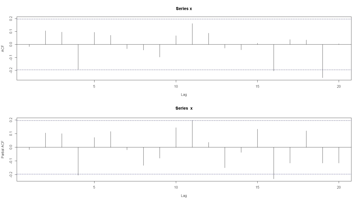
First of all, let’s simulate an univariate series under the Gaussian distributional assumption. By theory, this series has to be stationary.

> library(urca)
> library(forecast)
> library(normwhn.test)
> x <- rnorm(100)
> par(mfrow = c(2, 1))
> acf(x)
> pacf(x)
> whitenoise.test(x)
[1] "no. of observations"
[1] 100
[1] "T"
[1] 50
[1] "CVM stat MN"
[1] 0.8687478
[1] "tMN"
[1] -0.9280931
[1] "test value"
[1] 0.6426144
> x.adf <- ur.df(x, type = c("none"), selectlags = "BIC")
> summary(x.adf)

############################################### 
# Augmented Dickey-Fuller Test Unit Root Test # 
############################################### 

Test regression none 


Call:
lm(formula = z.diff ~ z.lag.1 - 1 + z.diff.lag)

Residuals:
     Min       1Q   Median       3Q      Max 
-1.75385 -0.60585 -0.03467  0.61702  3.10100 

Coefficients:
            Estimate Std. Error t value Pr(>|t|)    
z.lag.1    -1.008829   0.143635  -7.024  3.1e-10 ***
z.diff.lag  0.002833   0.101412   0.028    0.978    
---
Signif. codes:  0 ‘***’ 0.001 ‘**’ 0.01 ‘*’ 0.05 ‘.’ 0.1 ‘ ’ 1

Residual standard error: 0.9501 on 96 degrees of freedom
Multiple R-squared:  0.5064,    Adjusted R-squared:  0.4961 
F-statistic: 49.25 on 2 and 96 DF,  p-value: 1.909e-15

Value of test-statistic is: -7.0235 

Critical values for test statistics: 
     1pct  5pct 10pct
tau1 -2.6 -1.95 -1.61

> x.pkss <- ur.kpss(x, type = "mu", lags = "short")
> summary(x.pkss)

####################### 
# KPSS Unit Root Test # 
####################### 

Test is of type: mu with 4 lags. 

Value of test-statistic is: 0.4136 

Critical value for a significance level of: 
                10pct  5pct 2.5pct  1pct
critical values 0.347 0.463  0.574 0.739

> auto.arima(x, ic = 'bic')
Series: x 
ARIMA(0,0,0) with zero mean     

sigma^2 estimated as 0.8829:  log likelihood=-135.67
AIC=273.34   AICc=273.38   BIC=275.94

As shown in the above output:
1) Since x is simulated with the normal assumption, the series should be a white noise by definition.
2) ACF plot shows no auto-correlation at all, as it should.
3) In ADF test, the null hypothesis of unit root is rejected.
4) In PKSS test, the null hypothesis of stationarity is not rejected.
5) The output from auto.arima() suggests an ARIMA(0, 0, 0) model, which is completely in line with the assumption.

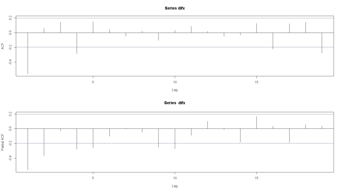
However, what would happen if we take the difference of x anyway?

> difx <- diff(x)
> par(mfrow = c(2, 1))
> acf(difx)
> pacf(difx)
> whitenoise.test(difx)
[1] "no. of observations"
[1] 99
[1] "T"
[1] 49
[1] "CVM stat MN"
[1] 1.669876
[1] "tMN"
[1] 4.689132
[1] "test value"
[1] 0.01904923
> auto.arima(difx, ic = 'bic')
Series: difx 
ARIMA(0,0,1) with zero mean     

Coefficients:
          ma1
      -0.9639
s.e.   0.0327

sigma^2 estimated as 0.901:  log likelihood=-136.64
AIC=277.27   AICc=277.4   BIC=282.46

The above output is quite interesting in a way that we just artificially “created” a model by over-differencing the white noise series.
1) After over-differenced, the series is not a white noise anymore with the null hypothesis rejected, e.g. p-value = 0.02.
2) In addition, the auto.arima() suggests that an ARIMA(0, 0, 1) model might fit the data.